


1. Introduction
Because of the operating conditions, a gear’s contact surface should be hard in order to be resistant to the contact wear and deformation, whereas the inner core needs to be tough in order to be resistant to crack propagation [1]. When placing a gear in a carbon-rich environment (carburizing) at high temperature in the austenitic range where carbon can diffuse into the steel, followed by rapid cooling or quenching in a quenchant (for example an oil), a zone close to the external surface undergoes a transformation to martensite. Further away from the surface the material does not undergo such a drastic cooling and has a lower carbon concentration, the austenite transforms to bainite, pearlite and ferrite.
During and after the carburization process followed by a heat treatment, because of inhomogeneous plastic deformations, the quenched specimen gets inevitably distorted [2]. These deformations are detrimental for the lifetime in operation of the gear, since higher deviations from the desired shape lead to higher out-of-balance forces. In large gears, corrective actions by means of material removal can be required. The most common way to deal with the distortions is by material removal after the quenching process. Since it is necessary for the gear to have a certain carbon penetration depth, one anticipates on the material removal by over dimensioning the carbon penetration in the carburization process. This is an expensive process since high temperatures and long times are involved [2]. Therefore, detailed knowledge of the heat treatment and the involved deformations is important.
In the case of large component gears, empirical methods (trial and error) are expensive because of the high material cost, and the complex testing strategy due to the numerous parameters that can influence the final result [3,4]. The aim of the current research is to investigate to what extent experimental tests on similarly shaped specimens on laboratory scale can be used to predict the deformations on real component scale, in terms of nature and magnitude. Therefore, 2 simulations have been done. They both investigate the same processes with similar times and temperatures, and the same material, but with different sizes. The first specimen has the real time geometry, whereas the lab-scale specimen has the real time geometry scaled with a factor 10.
The ability to deal with complex geometries and nonlinear material behavior makes the Finite Element (FE) method a suitable modeling technique for these kind of problems. Moreover, commercial FE software packages like ANSYS are compatible with CAD software [5]. Previous studies investigated stress and deformation development by coupling thermal, metallurgical, and mechanical fields for simplified geometries [6,7], or small samples [8]. Current research focusses on both large and small gears and includes effects that are typical for the 3 dimensional larger problems, like the gravitational effects, and the gear’s immersion time in the quenching bath. Decroos et al. showed how these effects, as well as the Transformation Induced Plasticity (TRIP) strain can be included in a commercial Finite Element software [9].
2. Specimen and Process
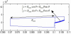
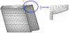
The real gear component under consideration is an involute gear with 48 teeth, an inner diameter of 70 cm, a root diameter of 100 cm, and a height of 30 cm. A two-dimensional cross section of a tooth is shown in Figure 1.
The total mass that has to be carried by 48 chains fixed at the gear is approximately 4100 kg. The chains are attached to the gear at hanging points located on the top surface in a symmetry plane of a tooth at one third from the root and two third from the inner diameter. The lab-scale specimen has exactly the same shape, but with all lengths 10 times as small as the real-time specimen. This means that there also 48 teeth, the inner diameter is 7cm, the root diameter 10 cm, and the height 3 cm. The total mass is approximately 4.1 kg.
In a carburization process, the material which is ferritic at room temperature, is heated in the austenitic stage and brought in a carbon rich gas environment, in order to promote carbon diffusioni into the material. After carburization the material is soaked [2], i.e.is hold on a slightly lower temperature, to allow further diffusion of carbon into the material. After soaking, the gear is quenched by immersing into an oil bath. Then the material is hold at a temperature around 150°C to decrease the brittleness of the martensite without significant loss of hardness. This process is called tempering. The time/temperature history of the carburization and heat treatment process is schematically shown in Figure 2.
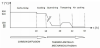
In the current process, the specimen is held for 10 hours at 950°C in a carbon-rich environment, is then soaked at a temperature of 920°C, and afterwards quenched in an oil bath of 90°C for 2 hours, followed by tempering at 150°C during 2 hours, and followed by 20 hours of air cooling.
The gear material is a case hardening steel, which means that is an acceptably soft steel with a high ability to form martensite upon quenching [10]. The alloying elements are Ni (1.8 wt%), Cr (1.08 wt%), Mn (0.9 wt%), and Mo (0.18 wt%). The initial carbon concentration is 0.19 wt%.
3. Numerical Procedure
3.1 Modeling the physical phenomena
3.1.1 Field problems and their couplings
The physical phenomena and their couplings that are present in a carburization and quenching process shown in Figure 2 are shown in Figure 3.
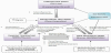
For every point of the specimen and throughout the whole process, the diffusion model solves the carbon concentration problem, the thermal model calculates the temperature, the metallurgical model the phase composition in terms of the volume fraction for each phase, and the mechanical model the stresses, strains, and displacements. The carbon concentrations are an input for a coupled thermometallo- mechanical model since they determine both the thermal and mechanical material properties as well as the transformation kinetics of the metallographic model. As shortly explained in Figure 3, the phase compositions, temperatures and temperature rates, and the strains and stresses each influence each other. More details can be found in reference [2].
3.1.2 Diffusion model
In the absence of body carbon generation sources, Fick’s law describes the evolution of the carbon concentration c(x,y,z,t) [1].
Hereby D is the diffusion coefficient, which is temperature dependent, but assumed to be independent of the carbon concentration.
The boundary condition on the surface layer determines to which
extent carbon is transferred into the material, and is dependent on
the carbon transfer coefficient hc, and the carbon potential C0 [2], as
shown in equation 2. The vector
3.1.3 Thermal model
A solution of a thermal analysis has to satisfy two basic laws, namely the conservation of energy and Fourier’s law of heat flow, which results in the heat equation 3.
Hereby T is the temperature (K), k the isotropic heat conduction coefficient (W/m), ρ the density (kg/m3), and Cv the heat capacity at constant volume, j a heat generation rate per unit of volume.
In a quenching process, there are no thermal heat sources, although
during phase transformations the latent heat of transformation can be
considered as a body heat source. If phase i transforms into a phase j
with a volume fraction transformation rate of
Hereby
Convection heat losses are described by the convective heat flux on the external surface boundary as given in equation 5.
Hereby h is the convective heat transfer coefficient
3.1.4 Phase transformation model
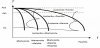
When cooling from the austenitic region, austenite can transform into martensite, bainite pearlite, and ferrite, or a combination of those phases, as shown schematically in the Continuous Cooling Transformation (CCT) diagram of Figure 4. For a certain carbon concentration and a given stress state (see Figure 2), the phase transformation behavior can be calculated based on the temperature history.
For diffusion controlled transformations, the time is divided in several discrete time steps and during each time step, the transformation or the incubation to transformation is considered to be isothermal. For the incubation time, Scheil’s additivity theorem states that transformation begins when the accumulated ratio of the time interval on the transformation starting time at that temperature from all previous time steps equals 1 [11].
Once the transformation of austenite started, each time step the transformed phase can be calculated by a Johnson-Mehl-Avrami- Kolmogorov (JMAK) relationship that describes the isothermal evolution of the i-th phase fi as a function of the transformation time tj as given in equation 7 [12].
For every temperature, the parameters a(T) and b(T) can be deducted from the Time Temperature Transformation (TTT) diagram, based on the times t0.01 resp. t0.99 on which 1% resp. 99% of austenite would be transformed when quenching to that temperature followed by holding. Both can be deducted from the TTT diagram. Based on equation 7, equation 8 gives the expressions for a(T) and b(T).
The transformation time tj from expression 7, can be calculated
based on the time step Δtj, equation 8, and the transformed phase of
the previous time step
The diffusionless martensitic transformation is described by a Koistinen and Marburger (KM) model that gives the volume fraction of martensite as a function of the temperature [13].
The temperature at which the martensitic transformation starts, Ms, can also be deducted from the TTT diagram. The influence of stress on the transformation behavior (see Figure 3), like for example the martensitic starting temperature Ms, is not considered in this analysis.
Influence of the carbon concentration on the transformation behavior (steels):
Carbon, together with most common alloying elements (except Aluminum and Cobalt), tends to move the TTT-diagram to higher times [10], in other words facilitating the martensitic transformation for the same (fast) cooling rate.
For a given alloy with a certain carbon concentration C, the transformation starting and finishing curves for each phase of the TTT diagram can be interpolated by a 2nd order polynomial giving the relationship between the logarithm of the time t as a function of the temperature T given by equation 11 [9]:
The phase transformation starting curves are found in reference [16] for 2 case hardening steels with the same alloying composition, except for the carbon concentration. The first steel has a carbon weight% of 0.2%, the second 0.97%, covering the range of concentrations observed in the investigated current work.
For an arbitrary carbon concentration, the coefficients ai(C) for a phase transformation starting curve are interpolated based on the coefficients for these steels and the carbon concentration. Since the output of the diffusion model is the carbon concentration, the procedure allows to obtain an analytical expression for all relevant starting and finishing lines of the TTT-diagram at any point in space.
3.1.5 Mechanical model
The total strain rate is an additive sum of strain rates [15]: the thermal, elastic, plastic, Transformation Induced Plasticity (TRIP) strain rate, and the phase transformation strain rate.
Thermal strain
For isotropic materials, the thermal strain is given in equation 13:
with αse the secant thermal expansion coefficient, Tref the stress-free reference temperature, δij the Kronecker delta.
Elastic strain
The relationship between stress and elastic strain is given by the generalised Hooke’s law of equation 14.
The fourth order tensor C is named the stiffness tensor, and has 2 independent constants in the case of an isotropic material, for example Young’s Modulus and Poisson’s ratio.
Plastic strain
Plastic strain rates are related to the plastic potential function [16] by formula 15.
Hereby Q is the plastic potential function in stress space and
equals the yield function when associated plasticity is assumed.
Phase transformation strain
Transformation strain is the strain due to the difference in unit cell
dimensions between austenite and the transformed phase [2]. Based
on the relative volume change between austenite and the new phase I,
Transformation Induced Plasticity (TRIP)
Transformation induced plastic (TRIP) strain is the irreversible strain, even under low stresses, when a phase transformation occurs [18].
Hereby fI is the transformed fraction, K is a constant, sij is the deviatoric stress. In reference [9], it is explained how to implement TRIP in a commercial FE software package.
3.2 Finite Element modeling
The geometry in the Finite Element model is constructed based on the mathematical equations of the lines and surfaces, that form the boundaries of the gear’s body. The non straight lines are created by means of cubic splines passing through nodes that have been defined based on the parametric expression of the line. The parametric equation of the involute line of the gear tooth of Figure 1, is depending only on the constants Rbase. Resizing Rbase with a factor 10 and using the parameter equation will automatically generate the equivalent line in the solid FE model of the lab-scale gear.
The specimen is meshed such that there is a mesh refinement in the direction where the highest gradients are expected. In both the diffusion, thermal, metallurgical and mechanical model, that direction is the normal to the external surface.
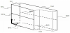
Because of symmetry it is sufficient to model only 1/48th of the total gear, as shown in Figure 5. The mesh of the real gear and the lab-scale gear consists of 213608 node brick elements and 24764 nodes, and is shown in Figure 5.
Perpendicular to the symmetry plane, which is in the tangential direction, there is a zero tangential carbon flow in the diffusion run, a zero thermal flux in the thermal run, and a zero radial displacement in the mechanical run.
As initial condition in the diffusion run there is a material carbon concentration of 0.19 wt%, in the thermal run the initial temperature is the soaking temperature. As a mechanical initial condition, it is reasonable to accept that the material is completely stress-free just before the quenching process [2]. The metallurgical initial condition is that the metal is initially fully austenitic.
The way to implement phenomena, such as the calculation procedure for the carbon concentration, Transformation Induced Plasticity, and gravity in a commercial Finite Element code has been explained in reference [9].
In 3D FE analysis, one commonly assigns a material to a volume of the solid model. Since in a FE solution procedure of any kind one has to calculate integrals over the entire volume [19] with material properties in the integrand, one can state [20]:
because the volume is divided in elements. Therefore, it is possible to define a different material law for every element [9,20]. In this analysis, every element’s material properties are dependent on the calculated element’s carbon concentration, and the element’s temperature and temperature history.
Temperature dependent material data for each phase are taken from reference [21]. A rule of mixture is used to calculate the properties based on the phase fractions.
4. Results and Discussion
The results of the diffusion model are the carbon concentrations in the specimen after the carburisation and soaking process. The results of the thermal run are the temperatures at every point in space starting from the soaking process, followed by quenching, tempering, and air cooling. The mechanical model calculates strains, stresses, and displacements after these processes. The results for both geometries are presented by means of line plots for the lines schematically shown in Figure 6.
4.1 Carbon concentration
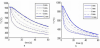
The carbon concentration after the diffusion process for both geometries is shown in Figure 7.
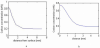
Both curves have a Gaussian shape with a comparable width at half maximum, and a comparable maximal value. The maximal carbon concentration at the outside surface is 0.83 wt% in the case of the realtime geometry, and 0.76 wt% in the case of the test geometry. The distance from the outer surface at which the carbon concentration is half of its maximal value is 1.4 mm for the real time case, and 1.35 mm for the test sample..In both cases, at 3 mm the concentration is the same of the initial bulk concentration of 0.19 wt%.
When considering the different length scales in mesh divisions, the small component has a ten times finer mesh than the large component. The similar results in both magnitude and shape for the final carbon concentration in the 2 specimens show that the prediction of the carbon concentration is not sensitive to the mesh density. The latter is thought to be due to the long times and the monotonous character of the carbon diffusion problem in the case of carburizing.
4.2 Phase composition
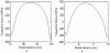
The martensite fraction after diffusion and rapid cooling for both geometries is shown in Figure 8.
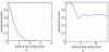
In the real-time geometry, the martensite volume fraction curve has a Gaussian shape, with a maximal martensite fraction at the surface of 92.6 %. The fraction drops to zero at approximately 3.2 mm depth. The martensite curve of the test geometry is completely different. That is due to the size effect which causes a more rapid cooling than in the large geometry case. The martensite fraction at the surface is 93.5% and eventually drops to approximately 65% at 4.5 mm. Note that for the test component the range of the graph of Figure 6b, namely 15 mm, is half of the size of the test component. The reason for the fluctuations in the curve is thought to be computational rather than physical.
4.3 Temperature
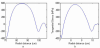
The temperature histories until 1 minute at several points of line MH2 (see Figure 5) are shown in Figure 9.
After 1 minute, the temperature difference between the surface and a point at 12 mm from the surface is approximately 180 °C for the large component, and 60 °C for the small component. At 12 mm depth, in the first case the temperature after 1 minute drops to 550 °C, and in the second case 300 °C. The latter is already beneath the martensite starting temperature of 415 °C for a carbon concentration of 0.19 wt%, which explains the martensite fraction of approximately 65% at that point, see Figure 9b.
4.4 Deformation/distortion/residual stress
The mechanical model predicts stresses, strains, and displacements after the quenching process. In the current work, the initial shape before the process is the same as the desired afterwards, which means the displacements of the surface can be considered as distortions.
The tangential residual stresses for both models on the 2 radial lines MH1 and MH2 (Figure 6) are shown in Figure 10.
For both models, except for the scaled ordinate axis, the stress curves have a similar shape and magnitude. The residual tangential stress is compressive at the outer surface of about 400 MPa, and has a higher tensile stress in the middle tending towards 600 MPa.
The tangential stresses on line MH2 are shown in Figure 11.
In both cases show again a very similar stress curve. Due to the gear tooth which lies along the line MH2, the profile is different from line MH1, see Figure 10. Away from the tooth (left of the curve), the same compressive stresses as on line MH1 are found, and more towards the centre, one has tensile stresses almost reaching 600 MPa.
The calculated displacements along certain lines (Figure 6) are shown in Figure 12.
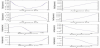
The larger component shows displacements in the order of tenths of mm, with maximum 0.7 mm, see Figure 12e. The small component shows displacements in the orders of hundreds of mm, with a maximum of 0.035 mm (Figure 12d).
The large model predict that a radial-axial cross section of the gear will have a barrel-type of deformation after carburization and quenching. The top and the bottom surface have a more complex deformation, as can be seen in Figure 12c and 12d. Again there is a clear difference in distortion prediction between the 2 models, with a difference reaching 1 mm. in the small case, since the outer vertical and horizontal radial respectively axial displacements follow more or less exactly the same tendency, the gear is rather rotated than deformed as a consequence of the quenching process. In general, the modeled deformations along the vertical lines show a good agreement with the experimental observations of a quenched hollow cylinder with similar inner and outer diameter to height ratio [22] for the large case, but not for the small case. This might be due to the fact that the martensite phase, which has a higher unit volume, see equation 16, has lower gradients throughout the specimen (Figure 12b).
5. Conclusions
A three-dimensional model to predict carbon concentrations, thermal histories, phase compositions, stresses, strains and displacements after a carburization and quenching process of gears has been used to investigate the differences between a large component gear, and a gear with exactly the same shape, but with length scales of a factor 10 smaller. Both specimens have undergone the same temperature cycle. The physical couplings have been incorporated in a diffusion FE model that models the carburization and soaking process, followed by a thermo-metallo-mechanical FE model that models the quenching process. Effects that become important when the size of the quenched components increase, namely gravity and immersion time, have been taken into account in both cases.
The results of the diffusional models show a similar carbon concentration profile and magnitude for the large component and the test component. As both FE meshes consist of a similar number of elements, and considering that the difference in length scales, it can be concluded that the carbon concentration calculations in carburization and soaking processes are mesh insensitive.
The thermal results show, as expected, faster cooling rates for the lab-scale specimen than for the large component gear. The implications for the metallurgical transformations are such that the nose of the bainite transformation is avoided, and martensite forms through the entire lab-scale specimen, whereas the martensite penetration is in the order of millimeters in the large component gear.
The quenching stresses, which are the causes of the deformations, show a very similar magnitude and profile for the large component and the lab-scale component when scaling the length coordinate. However, the deformations are of a completely different nature. From this study it can been concluded that the deformation behavior after carburisation and quenching of a lab-scale component can not be extrapolated to a larger scaled component when the length scales are of a different order. However, the residual stress profiles are independent of the component’s size.
Competing Interests
The authors declare that they have no competing interests.