


1. Introduction
Quadrotor aerial vehicles are highly maneuverable and have enabled a number of indoor and outdoor applications, e.g., three-dimensional (3D) environment exploring, mapping, navigation, transporting, military and commercial opportunities. The ability of 3D movement brings great research interest in the field of mobile robotics.
Corke [1] provides a comprehensive introduction to the 3D dynamics model of quadrotor robots using Newton’s second law and Euler equations. And a PID-based inner-loop/outer-loop scheme is proposed for the 3D translation and yaw control. Mahony et al. [2] propose a tutorial introduction to the rigid-body dynamics modeling, estimation, and control for multirotor aerial vehicles including the quadrotor case. They also give a physical discussion about the rotor blade flapping referring to [3,4], and then presented a disturbed external force model due to the blade flapping effect. Beard [5] considers the problems of dynamics, state estimation, and control of a quadrotor aerial vehicle.
In Yesildirek et al. [7], the quadrotor system is decomposed into three fully actuated subsystems in pitch, roll and yaw domains. They propose a multi Lyapunov function based switching control algorithm to achieve tracking of Cartesian space motion and the heading angle of the quadrotor. Hao et al. [8] propose a change in describing the dynamics of the quadrotor and separate the dynamics into three sub-groups. Then combined with a coordinate transformation, they propose a trajectory tracking control design using the backstepping technique. Zhao et al. [9] present an asymptotic tracking controller for the quadrotor using the robust integral of the signum of the error (RISE) method and an immersion and invariance (I&I)-based adaptive control methodology. The proposed control system is composed of two parts: the inner loop for attitude control (using the RISE approach) and the outer loop for position control (using the I&I adaptive control methodology. The proposed control system is composed of two parts: the inner loop for attitude control (using the RISE approach) and the outer loop for position control (using the I&I approach).
This paper will consider the 3D dynamics modeling of the quadrotor with blade flapping effect via the Newton-Euler approach and the position and yaw angle trajectory tracking control design using the backstepping technique. Computer simulation is conducted to illustrate the trajectory tracking performance of the 3D translation and yaw motion.
2. Dynamics Model of a Quadrotor Robot
Refer to Figure 1, the quadrotor robot comprised of a main frame
structure and four blade rotors (numbered 1, 2, 3, and 4 clockwise) is
considered as a rigid body, where the body coordinate system {B} is
defined with its origin G attached to the center of mass of the whole
robot, and the inertia (world) coordinate frame {W} with origin
at O is fixed on the earth surface. The positive direction of axis is
defined along the heading direction of the vehicle. Rotors 1 and 3
rotate clockwise, and rotors 2 and 4 rotate counterclockwise. In the
dynamics modeling, we consider the gravity force along the negative
Zw direction, and the four thrust forces
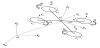
where l is the distance from the center of mass G to each rotating axis.
ZYX Euler angles (ψ, θ, ϕ) are used for representing the orientation
of the quadrotor vehicle’s body frame with respect to the world frame
Where
Define t = [x,yz]T as the position vector of the center of mass G of the quadrotor robot in terms of the world frame, and assume that the robot structure is symmetrical about the coordinate system. Consider the quadrotor robot being under normal flight conditions, i.e., the roll and pitch angles are very small, and the flight drag force is negligible. By the Newton’s second law and Euler equations of motion, we can derive the dynamics model of the quadrotor robot as follows: [1,14]
where m is the mass of the quadrotor robot, g is the gravitation acceleration constant, I = diag[Ixx, Iyy, Izz] is the mass inertia matrix about the body frame {B}, Ixx, Iyy, and Izz are the moments of inertia about ZB axes, respectively.
Mahony et al. [2] considered the blade flapping effect and proposed
a simplified flapping model. Neglecting the effect of the vertical
velocity component, we consider the quadrotor robot being with a
flight velocity vector νB = [u, ν, 0]τ. In order to simplify the flapping
model, the four rotors are assumed with same conditions. The
aerodynamic disturbance forces resulting from the deflection of the
rotor blades in the XBYB plane can be derived as follows. As shown in
Figure 2, define the flapping angles β and
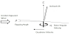
where β is the tilt angle of the rotor away from the incoming
apparent wind, and
Define the sensitivity matrix Aflap of the flapping effect to the apparent wind:
then the total force acting on the quadrotor robot can be represented as:
Substituting Aflap and Equation (4) into Equation (5), the translational equations of motion of the quadrotor robot can be derived as follows using the Newton’s second law:
where α = atan2(ν,u) is the angle between the velocity vector υs and XB axis. And the rotational equations of the robot are still expressed by Equations (2b).
3. Adaptive Control via Backstepping for Quadrotors with Blade Flapping
Since a quadrotor aerial vehicle has only four rotor actuators, it is an underactuated system and difficult to control it to have arbitrary six degrees-of-freedom motion in the free Cartesian space. Due to the limit of only four rotors, it is natural to choose the four important motions including the three translational components and the heading rotation (i.e., the yaw angle) as the control objectives. That is, we can set four arbitrary desired trajectories: xd(t), yd(t), yd(t) and ψd(t), and propose a suitable stable control law to obtain the trajectory tracking control objective.
In this paper, we will propose a nonlinear stable adaptive control design using the backstepping approach [6,15] for quadrotor robots considering the blade flapping effect. Based on the dynamics model: Equations (6) and (2b), and after substituting (1) into the model, we can first define the following four control input variables:
and choose the state vector
and the unknown flapping angles vector as:
Equations (6) can be expressed as the regression model:
where
And
In the derivation of stable adaptive control law, the estimate of
the unknown flapping angles is defined as
3.1 Z-axis motion control design
First, consider the
Define the tracking error
where Zd(t) is the desired trajectory for .Taking the time derivative, we have:
Choosing Lyapunov function candidate as:
we can obtain the time derivative as follows:
By choosing the virtual input
we have
Consider the subsystem:
And define
we can obtain:
Choosing Lyapunov function candidate:
and taking the time derivative, we have:
Hence, we can choose the control law:
and obtain:
3.2 x-axis subsystem control design
Similarly as the z-axis design procedure, the x-axis subsystem can be
considered by introducing the virtual inputs
where xd(t) is the desired trajectory for x. Choose Lyapunov function candidates:
After taking their time derivatives and choosing β2 and βux as:
we can obtain:
3.3 y-axis subsystem control design
Similarly, the y-axis subsystem can be considered by introducing the virtual inputs β3, βuy for x8 and uy respectively, and defining the errors:
where Yd(t) is the desired trajectory for y. Choose Lyapunov function candidates:
After taking their time derivatives and choosing β3 and βuy as:
we can obtain:
Flapping Angles Estimator Design
Choose Lyapunov function candidate:
where Γ is a 2×2 positive-definite weight matrix. Taking the time
derivative and substituting into U1, βux, and
Thus, we can choose the unknown flapping angles estimator as:
and obtain
Since
4. Pitch Subsystem Control Design
Consider the pitch subsystem and introduce virtual input β for x11. Define the error
and choose Lyapunov function candidate:
In order to make the time derivative
where
Define the error
In order to make the time derivative
5. Roll Subsystem Control Design
Consider the roll subsystem and introduce virtual input input βϕ for x10. Define the error
and choose Lyapunov function candidate:
To make
Define the error
In order to make the time derivative
6. Yaw Subsystem Control Design
Finally, consider the control of the yaw subsystem:
First, introduce the virtual input β4 for x12, and consider:
Define the yaw tracking error:
where
After taking the time derivative
we can obtain:
Then define the error
and choose Lyapunov function candidate:
After taking the time derivative
we can obtain:
Thus, the closed-loop yaw subsystem is asymptotically stable.
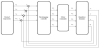
The proposed overall control system for a quadrotor robot can be summarized as shown in Figure 3.
7. Computer Simulation and Discussion
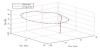
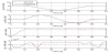
The tracking performance of the proposed adaptive control system with flapping compensation is tested via computer simulation using Matlab/Simulink as shown in Figure 3. Consider the desired trajectory created using the cubic spline method as shown in Figure 4. The quadrotor is requested to flight straightly up to a height of 4 m from the origin of the world coordinate system in 10 seconds, and then move counterclockwise in a circle with radius 5 m keeping the same height in 50 seconds. Then the quadrotor is required to maintain a steady hover in the final 10 seconds. The yaw angle is kept constant at in the whole flight.
In the simulation study, the parameters of the quadrotor robot are selected as follows m=0.8 kg, r=0.1 m, g=9.81 m/s2 , l =0.5 m, A1c = A15= 1.5,
The parameters of the controller used are as follows:
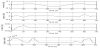
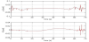
The three-dimensional tracking result of the whole trajectory is shown in Figure 4. The trajectory tracking in the , , and axes and the yaw angle tracking are shown in Figure 4.1. The tracking errors are shown in Figure 4.2. The induced roll and pitch angles during the flight are shown in Figure 4.3. Equation (7) describes the relation between the control variables and the squared rotor speeds. Using the inverse transform we can find the required squared rotor speeds corresponding to the control signals In order to get all positive the parameters of the controller must be suitably chosen. In this work, the response in the y-axis is thus lagged the desired trajectory approximately from s and has larger tracking error and the largest tracking error is approximately 0.23 m. From Figure 4.3, we know that the roll and pitch angles are small and reasonable, thus the flight is stable. The largest tracking errors in the and z axes are approximately 0.05 m and 0.02 m, respectively. The yaw angle can be kept at as shown in Figures 4.1 and 4.2. Figure 4.3 shows that in order to keep steady hovering, the required roll and pitch angles are larger during the hovering period. The estimates of the flapping angles are shown in Figure 4.4, and the estimate errors are larger in the hovering period.

8. Conclusion
This article considers the dynamics modeling and nonlinear stable adaptive control design with blade flapping compensation for the quadrotor robots. The quadrotor robot is under-actuated since it has only four rotor actuators for three-dimensional flight maneuvering. It is rather difficult to construct an arbitrary six- dimensional flight control, so the usual approach to the control design adopts only the three-dimensional translation and yaw angle tracking control. The dynamic x-axis motion of a quadrotor could be induced by suitable small pitch rotation, and the y-axis motion could be affected by the roll motion. Based on these characteristics, this paper proposes a backstepping-based stable adaptive control design considering the blade flapping effect. Computer simulation is conducted to illustrate the trajectory tracking performance of the 3D position and heading control. The roll and pitch angles generated by the controller are small enough, so the flight is stable and reasonable. In the simulation, the choice of the controller parameters is compromised for getting positive squared rotor speeds to compute practical rotor speed commands.
Competing Interests
The authors declare that they have no competing interests.
Author Contributions
All the authors substantially contributed to the study conception and design as well as the acquisition and interpretation of the data and drafting of the manuscript.