


1. Introduction
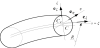
The majority of the textbooks on strength of materials deal with curved beams made of homogeneous material. Formulae are presented for the calculation of the normal stress, the shearing stress, the change of curvature and the strain energy stored in the curved beam. In this paper our main objective is to generalize these classical results for a curved beam made of heterogeneous isotropic materials By assumption the elastic parameters, i.e., the Young modulus and the Poisson number, depend on the cross sectional coordinates, but are independent of the axial coordinate. Figure 1 shows a part of the beam and the applied orthogonal curvilinear coordinates. Our most important assumptions are as follows:
- The displacements and deformations are small;
- The curved beam has a uniform cross section and a constant radius;
- The cross section is symmetric with respect to the axis ζ;
-
The Young modulus E and the Poisson number v satisfy the
following relations:
- The Young modulus is the same in tension and compression;
- The magnitude of the normal stress σξ is much greater than those of the stress components and σζ;
- The temperature is constant (there is no heat effect).
These assumptions are associated with the displacement hypotheses detailed in the following section.
2. Displacement Hypotheses
The orthogonal curvilinear coordinates are shown in Figure 1. We shall assume that (a) the crosssections are symmetric with respect to the axis [consequently the beam is symmetric with respect to the coordinate plane (ξ = s, ζ)] (b) the E-weighted first moment of the cross section with respect to the axis – this quantity is denoted by Qen – is equal to zero:
The axis ξ = s intersects the plane of the cross section in the point Ce, which is referred to as the E-weighted center of the cross section (in contrast to the point C, which is the geometrical center of the cross section).
The coordinate line ξ = s is the E-weighted centerline (or centerline in short) of the curved beam, and s is the corresponding arc coordinate.
We next introduce the concepts of E-weighted area and moment of inertia with respect to the axis
These concepts have been introduced for a straight beam in paper [1] by Baksa and Ecsedi.
The unit tangent vectors eξ(s), en and eζ(s) of the coordinate lines ξ, n, and ζ are also shown in Figure 1. Let R be the radius of the E-weighted centerline. It is easy to check that eξ(s), and eζ(s) satisfy the following relations
It is also obvious that the operator Δ takes the form:
We shall assume that (a) the cross section has a translation and a rigid body rotation about the axis , i.e., it remains a plane surface during the deformation, and (b) the deformed centerline remains perpendicular to the cross section. Under these conditions
is the displacement field on the cross section, in which uo = uo eξ +
wo eζ and
is the rigid body body rotation. Consequently
from where
and
Since
where at least one factor in the dyadic products denoted, for brevity, by ((...)) is perpendicular to eξ, we have
Here
are the axial strain and the curvature on the E-weighted centerline.
2.1 Formulae for the normal stress
Generalization of the Grashof formula. The E-weighted reduced area, first moment and moment of inertia are defined by the following relations:
It is clear that the axial force and the bending moment are
Here, due to the inequality
As for the bending moment, in a similar way we obtain
After solving equation system (13) we have Є0ξ and κ0 in terms of the axial force and the bending moment:
Let us now substitute these solutions into equation (9) so that we can get the axial strain:
With the knowledge of the axial strain
is the normal stress.
In what follows, we attempt to simplify the above formula for the normal stress. First we shall clarify how AeR, QeR and IeR are related to Ae, Qen and Ien. Using the power series of fraction R/ (R + ζ) we have
and
because Qen = 0. For the denominator in equation (16) the following approximation holds
since
Using this result we can rewrite formula (15):
If we use approximations (17) we can check the following equations
Substituting the last two formulae into (20) and the result into the Hooke law we have
This formula is the generalization of the Grashof formula for the case of cross sectional inhomogeneity
A formula for the normal stress assuming pure bending. English
textbooks contain a formula for the normal stress under the
assumption of pure bending – see for instance equation (4.71) p. 224
in [2]. In this subsection it is our aim to generalize the cited equation
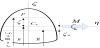
for heterogenous curved beams. Figure 2 shows the cross section
and the geometrical meaning of some notational conventions: ζo is
the coordinate of the neutral axis with radius
is the formula for the normal stress. We would like to manipulate it into a form similar to the one cited above.
First we shall determine the location of the neutral axis. It follows from condition σ3 = 0 which needs to be satisfied on the neutral axis that
Consequently
from where
is the radius that belongs to the neutral axis. Upon substitution of AeR and QeR from (11), the radius R of the neutral axis assumes the form
or equivalently
For E(η, ζ ) =constant, the above equation coincides with formula (4.66) p. 222 in [2]. Now we shall proceed with the determination of the normal stress. Using equation (26), the factor in parentheses in equation (23) can be rewritten into the form
If we use the inequality
The last open question is how to transform the fraction R/IeR into a suitable form. The following equation details the transformation step by step:
It is worth introducing the notation e = -ζo. Upon substitution of the result obtained into formula (29) for the normal stress we arrive at its final form:
This equation is the generalization of formula (4.71) p. 224 in [2] valid for the homogenous case for curved beams with cross sectional inhomogeneity.
2.2 A formula for the shear stress
Our goal in this subsection is to derive a closed form solution for calculating the shear stress. We shall use equilibrium equations for this purpose. This approach results in a relatively simple formula; however, it has the disadvantage that the kinematic equations are not satisfied. The basic idea is well known from the theory of straight beams: we divide a short portion of the beam into two parts and then analyze the equilibrium conditions of one part.
Consider Figure 3 which shows a finite portion of the curved beam with cross sectional inhomogeneity. The left cross section with arc coordinate sB is fixed, coordinate s > sB of the right cross section is regarded as a parameter. We shall use the following assumptions:
- The shear stresses τξ = τηξeη + τζξeζ on the line ζ = ζ = constant intersect each other in one point which coincides with the intersection point of the tangents to the contour of the cross section at ζ = ζ = constant. Consequently, τηξ = -τηξ(-η), which means that τηξ(η) is an odd function of η.
-
The shear stress τηξ is constant if ζ = constant.
The bending moment M and the shear force V are related to
each other via equation
which is an equilibrium condition.
- The normal stress σξ can be calculated by equation (22) for which we assume N = 0 – there is no axial force in the cross section considered.
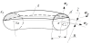
For calculating the shear stresses τηξ let us consider the part of the
beam with outlines drawn thick in Figure 3. It is bounded by the
marked endfaces
The equilibrium equation for the part of the beam considered is of the form
If we take into account that the shear stress -
is the surface element, then it follows that the last integral in (33) is the resultant of the shear stresses.
Let us differentiate equation (33) with respect to s. Then (a)
substitute the derivatives of the unit vectors eξ and eζ with respect to s;
(b) take into account that (1) the integral over
If we now dot multiply throughout by eξ we obtain
Let emax be the distance of the top of the cross section from the point
Ce. This is always less than R. The area A' can be given as a product
is an upper limit of the second integral in (34). Really if we take into
account that the shear stress is taken on the line
for the calculation of the shear stress
Upon substitution of the normal stress from (22) – N = 0 by assumption – we have
A further transformation yields
Introducing the notations
and
and substituting (32) we obtain
which is a formula for the average value of the shear stress. This result is a generalization of a classical formula valid for curved beams made of homogenous material – see pp. 358-359 in [3, 2002].
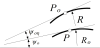
2.3 Curvature change, strain energy
In the present subsection [the radius of curvature] {a point} on the E-weighted centerline before and after deformation are denoted by [Ro and R] {Po and P}. The angle formed by the tangent to the E-weighted centerline at Po with the horizontal axis is ψo. Its change during deformation is ψoη – the rigid body rotation. The calculation of the curvature change is based on Figure 4 which shows all the quantities mentioned.
The infinitesimal arc element dso on the E-weighted centerline before deformation changes to ds. It is clear that
is the axial strain on the E-weighted centerline. Consequently
Using the above equation we can manipulate the formula for the curvature change:
Here
A comparison of equations (10), (42) and (43) yields
Substituting ĸo from (14) and taking into account that in the present
case N = 0 and
that is
Now we proceed to determine the strain energy stored in the beam. It is not too difficult to check using equation (45) that the angle change dψ due to the bending moment is
Consequently
is the work done by the bending moment exerted on an infinitesimal portion of the beam. Let L be the length of the E-weighted centerline. After integration
2.4 Numerical examples
Example 1. Figure 5 shows the cross-section of the curved beam considered. We assume that the beam is subjected to pure bending M = M eη ; M = 100 Nm. The geometric dimensions are all given in Figure 5. The lower part of the beam is made of steel and the upper part of the beam is made of aluminium. The corresponding material parameters are E1 = 2:1×10⁵ MPa and E2 = 7 ×10⁴ MPa, in that order. Our aim is to depict graphically the normal stress distribution as a function of ζ using the three formulae derived in the previous sections. This allows us to compare the various results. It would also be interesting to check the difference between these formulae regarding the radius of the neutral axis.
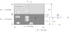
First we determine the ordinate zC of the E-weighted centerline in coordinate system γz. Since the E-weighted first moment of the cross section with respect to the axis η should be zero, the following equation holds:
Consequently
With the knowledge of zC one can read off from Figure 5 that
Before computing the stresses sought we shall set up appropriate formulae for the E-weighted geometrical quantities AeR, QeR, Ieη and IeR. Recalling equation (11)1 we can write
Regarding the E-weighted reduced first moment of the crosssection, equation (11)2 yields
Using the parallel axis theorem, we can determine Ieη as
Therefore, recalling (11)3 and utilizing equation (54) we can establish a formula for the E-weighted reduced moment of inertia:
Substituting now a, b1, b2, R, A1, E1, A2, E2, ζk, ζ-1 and ζ+2 into equations (52)-(55) we obtain the following numerical values:
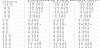
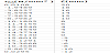
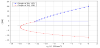
With these results we can compute the normal stress 6 using Eqs. (16) – this formula has no simplifications, it is exact under the displacement and stress hypotheses –, (22) – this is a generalization of the Grashof formula – and (31) – this a generalization of the formula that can be found in English textbooks on Strengths of Materials. The computational results are presented in Table 1 and graphically in Figure 6. It is clear that the results obtained by the use of the Grashof formula and by Eq. (31) almost coincide.
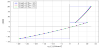
As regards Figure 6 the graphs representing the exact solution, the solution obtained by the use of Eq. (22) and the solution calculated with Eq. (31) are drawn in blue, red and green. Observe that the red and green curves coincide almost completely.
As for the ordinate of the neutral axis, by setting
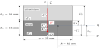
Example 2. Figure 7 shows a cross-section of the curved beam considered - observe that the beam is the same as in the previous example. Let us assume that the cross-section is subjected to a shear force V=10kN. The shear stress can be calculated using Eqs.(38) and (39). Upon substitution of and (56)2,5 into (38a)1 we have
We get in the same way that
With
Consequently
The values in Table 2 are computed using equations (57) and (58).
We should remark that formula (39) for the shear stress provides an average value – it has been established by using equilibrium conditions. Consequently, the values obtained using this equation are in all probability more accurate if the modulus of elasticity is independent of η, i.e., if it depends on ζ only.
3. Conclusion
In this paper we have generalized some classical results valid for curved beams made of homogeneous and isotropic material for the case when the curved beam is made of heterogeneous and isotropic material, under the assumption that the elastic parameters, i.e., the Young modulus and the Poisson number, depend on the crosssectional coordinates, but are independent of the axial coordinate. We remark that the Poisson number has played no role in the investigations.
By applying the well known displacement hypotheses we have established (1) three formulae for calculating the normal stress, (2) a formula for the shear stress, and (3) formulae for the change of curvature and the strain energy stored in the beam.
Except the very first formula for the normal stress -- see Eq. (16) -- all the others are generalizations of classical results and each can be applied in paper-and-pencil calculations.
Two numerical examples are presented to illustrate the applicability of the formulae.
Competing Interests
The authors declare that they have no competing interests.
Author Contributions
Both the authors substantially contributed to the study conception and design as well as the acquisition and interpretation of the data and drafting the manuscript.