


1. Introduction
The New Madrid Seismic Zone (NMSZ) represents the most hazardous seismic zone in the central and eastern US.
The great earthquakes of 1811-1812 caused extensive ground failures (especially liquefaction), and evidence of this phenomena can be seen even today on satellite images.
The great thickness of the soil sediments has been the focus to study the amplification or de-amplification given input strong ground motions with PGA > 0.4g due to degradation of shear moduli and increase of strains in depth.
The sites under investigations are located in the NMSZ on the Mississippi embayment, characterized by very thick sediments (730- 780m) overlying the Paleozoic rock [1-3].
The upper part of these deep sediments (80m) consists of very poor Quaternary deposits, studied by SASW and cross-hole techniques [1-3].
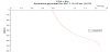
As there are no strong motion records in this area, therefore synthetic ground motions were used (Figure 1).
This paper focuses on the engineering significance of the geophysical method used for the purpose ground response analysis assuming that the resolution and quality of SASW data would be sufficient for the purpose of ground response analysis in shallow and deep soil deposits such as the ones present in the NMSZ.
Author of this paper participated in FHWA project for bridges in NMSZ with a research team of Missouri S&T, in Rolla.
2. Seismic Activity of New Madrid Zone (NMSZ)
2.1 Maximum expected magnitude according to statistical data
Generally it’s known that
the size of small earthquakes(M < 6.5) is better measured by body wave magnitudes (mb), (saturated at the value about 6.5).
Based on the earthquake catalogue for the period 1795-1995 for New Madrid Zone [3], all the magnitudes are given as body wave magnitudes (mb).
2.2 Conversion of mb magnitudes to Ms magnitudes
For NMSZ all mb magnitudes were transformed to Ms magnitudes according to the relationship [5]: mb = 0.56Ms + 2.9 (Table 1).

It can be seen that cumulative relationships: logN(mb) and log N(Ms) are more reliable (greater coefficients of correlation (0.963 & 0.969) and b-values are very small (b = 0.30-0.35) which confirms very high tectonic activity of NMSZ.
2.3 Non-cumulative and cumulative plots logn(Ms) &log n(mb)
According to non cumulative graph log n (Ms) relationship it can be observed that:
The minimum magnitude to be considered should be mb = 4.4 (Ms = 2.8) (Figure 2).
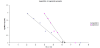
Non-cummulative log n(Ms) = a-bMs graph show Msmax = 6.3
Non-cummulative log n(mb) = a-bmb graph show mbmax = 6.0
According to cumulative graph log N(Ms) the minimum magnitude to be considered should be mb = 4.4 (Ms = 2.8) (Figure 3).
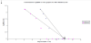
Cummulative log N(Ms) = a-bMs graph show Msmax = 7.0
Cummulative log N(mb) = a-bmb graph show mbmax = 6.8
The expected maximum earthquake following the linear extrapolation of cumulative plotts for NMSZ should be ~ Ms = 7.0.
2.4 Maximum expected magnitude according to seismic intensity data for the New Madrid earthquakes of 1811-1812
As can be seen from the log n(Ms) graph there is a lack of data for magnitudes mb = 5.5 - 7.5 or Ms = 4.7 - 8.2.
As at the time when New Madrid earthquake occurred were no instruments, the most reliable data are those on seismic intensities felt during this earthquake, which was felt widely in CEUS.
There are a lot of publications concern this problem, but we took into consideration two of them [7,8].
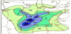
2.5 The generalized isoseismal map of NMSZ earthquakes
The isoseismal map of the shock of December 16,1811, is characterized by an unusually large felt area, with intensities of V as far away as the southeast Atlantic coastal area.
2.6 Assessment of the magnitude of New Madrid earthquakes from seismic intensities
The size of large ones (M > 6.5) is better measured by Ms especially for those in the range 6.5 - 8.0, but saturates above that value
The assessed expected maximum earthquake following the linear extrapolation of cumulative plotts should be about:
Ms = 7.0 - 7.5
which coincides with the seismic intensity MM = VIII according to the isoseismal map, but there are differences from 8-11 degrees.
For very large earthquakes was proposed “moment magnitude "Mw" [9].
Mw = Ms= (2/3)log10 Mo-10.7
where: Mo is seismic moment
Then expected maximum earthquake for NMSZ should be at least
Mw = 7.0 - 7.5
3. Near-Fault Earthquake Effects for Highway Bridge sites in NMSZ
3.1 Synthetic ground motions used as input - Point source model
3.1.1 Geotectonic model
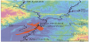
The Bridges sites under investigation are situated on the top of thick sediments overlying the Reelfoot Rift in New Madrid Zone.
The bridges are part of the located alongI-55 highway in the southeast corner of the state of Missouri near the cities of Hayti and Steele (Figure 5).
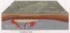
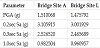
3.1.2 Depth to bedrock
For the determination of the depth to Paleozoic bedrocks the data from MoDNR [1] were used (Table 2).
- Ground surface approximate elevation (m)
- Base of Unconsolidated Alluvium Approximate Elevation (m)
- Approximate Depth to Base of Unconsolidated Alluvium (m)
- Approximate Thickness of Unconsolidated Alluvium (m)
- Top of Unconsolidated Tertiary& Cretaceous Sediments (m)
- Approximate Depth to Top of Unconsolidated Tertiary& Cretaceous Sediments
- Approximate Thickness of Unconsolidated Tertiary & Cretaceous Sediments (m)
- Top of Paleozoic Bedrock. Approximate Elevation (m)
- Approximate Depth to Top of Paleozoic Bedrock (m)
- Approximate Thickness of Paleozoic Bedrock (m)
- Top of Precambrian Basement (m)
- Approximate Depth to Top of Precambrian Basement (m)
- Approximate Bottom of Seismogenic Crust (km)
3.1.3 Modification of strong ground motions generated by the Reelfoot Rift by geological conditions
The thickness of soil layer on the top of hard Paleozoic rocks was derived from the data supplied by MoDNR (Table 2):
- Top of Paleozoic bedrock at depths: h = -700m 9L site) and h = -650m (A site) behaving linearly
- Thickness of consolidated sediments: H = 700m (L site), H = 650m (A site)
- Approximate thickness of unconsolidated alluvium and Tertiary sediments: H = 55 + 25 = 80m (L site), H = 55 + 25 = 80m (A site) studied by SASW and CH techniques behaving nonlinearly. That may cause the amplification or de-amplification for PGA > 0.4g due to degradation of shear moduli and increase of strains in depth
- The great earthquakes of 1811-1812 caused extensive ground failures (especially liquefaction). Evidence on satellite images
- As there are no strong motion records in this area, the synthetics as input motions were generated at the top of consolidated sediments overlying the Paleozoic bedrock
3.2 Results of a study using the Point-Source Model
3.2.1 Shear wave velocity (Vs) models
For the generation of synthetic ground motions the velocity models for Mid-America & NMSZ according to the inversion of teleseismic data were used [10], so named Soil USGS96 source model (M5).
The preliminary sediment thickness for the model was 1000m thick for New Madrid Seismic Zone (Table 3).

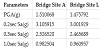
3.3 Strong Motion Parameters according to Seismic Hazard Maps
According to the USGS seismic hazard maps for PE = 2% in T = 50yrs, by entering a latitude and longitude for A, and L bridge sites at the USGS-National Seismic Hazard Mapping Project the strong motion parameters listed in Table 4 can be deduced.
The distances and magnitudes used to calculate these hazard values were found according to the USGS special tables for PGA, 0.2 sec Sa, 0.3 sec Sa and 1.0 sec Sa, as functions of log (km) and moment magnitude (Mw).The synthetics for both bridge sites were generated for three combinations of parameters were chosen, as
D = 10km & Mw = 7.1
D = 16km & Mw = 7.8
D = 20km & Mw = 8.1
3.4 Computer codes
For generating synthetic motions, Boore’s SMSIM package [11] is used in which: using input data were MW, D(km), h(m), number of simulations, and seed number, were computed acceleration time history, peak motions (PGA, PGV, PGD), and response spectra for a given damping (5%).
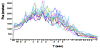
3.5 Acceleration time histories (Synthetics) [12]
Synthetics used as input motions were generated for different thickness of sediments (H) on the top of consolidated sediments overlying the Paleozoic bedrock.
3.5.1 Synthetics for H = 0m
Correspond to generation of synthetics on free surface of rocks.
3.5.2 Synthetics for H = 650m
Synthetics were generated for the thickness h = 730 - 80 = 650m.
Acceleration time histories and velocity time histories were computed for 5 random values (seeds) (123, 1234, 2345, 345, 78).
For each of three combinations of distances and magnitudes
D = 10km & Mw = 7.1
D = 16km & Mw = 7.8
D = 20km & Mw = 8.1
were generated 15 synthetics (Figure 6).
3.5.3 PGA values
3.5.3.1 Dependence of synthetic PGA values from H (m)
From the figure 7 it can be seen the decrease 2 times of PGA values on bedrocks (at H = 650m) to free surface (H = 0m).
3.5.3.2 PGA values for H=0m (on the top of Paleozoic rocks)
It’s the common case of the generation of synthetics on hard rocks, taking the thickness of overlying layer H=0m.
As an example are presented 3 synthetics for the same Seed=123 for different magnitudes and distances (Table 5).
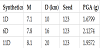
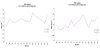
3.5.3.3 PGA values for the thickness of H=650m
PGA & PGV values for 15 synthetics for each bridge site are close to each other (Figure 8).
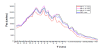
3.5.4 Sa spectra
3.5.4.1 Synthetic Sa spectra for different thickness H of sediments on the top of Paleozoic rocks
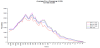
The maxims of Sa spectra of synthetics are displaced to the longer periods and decreasing as values with the increasing of thickness of sediments (H) (Figure 9).
3.5.4.2 Sa spectra for 5 random values for different combination of Mw and D (km)
Average values of Sa spectra for 5 random values for different combination of Mw and D (km) are close to each other with the lowest values for Mw = 7.1, D = 10km and the highest ones for Mw= 7.8, D= 20km (Figure 10).
3.5.4.3 Sa spectra for synthetics with H=650m
Sa spectra for 5% damping value of synthetics generated for H=650m are presented in the Figure 11.
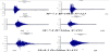
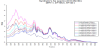
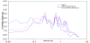
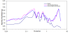
3.5.4.4 Comparison of Sa spectra for synthetics with H=0m &H=650m
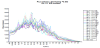
Sa spectra for H = 0m (blue lines) are characterized by the highest response values versus smaller periods (0.04-0.16sec).
Sa spectra for H = 650m) (red lines) have the lower peak values versus medium periods(0.25-0.55sec) (Figure 12).
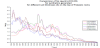
3.5.4.5 Comparison of Sa spectra for synthetics with H = 650m for point source model with those for composite model
From Figure 12 it can be seen that the average Sa spectra (D = 0.05) for both Point Source (H = 650m) (red line) and Composite Model (blue lines) are very close to each other concerning the shape, but they differ concerning the amplitudes.
3.6 Strong Motion Parameters According to NEHRP Maps
The USGS 1996 seismic hazard maps for PE = 2% in T = 50yrs by entering a latitude and longitude for two bridge sites at the website of National Seismic Hazard Mapping Project [10] were used to find the corresponding seismic hazard parameters (Table 6).
The distances and magnitudes used to calculate these hazard values were found according to the USGS special tables for PGA, 02.sec Sa, 0.3 sec Sa and 1.0 sec Sa, as functions of log (km) and moment magnitude (Mw). To generate synthetics for both bridge sites three combinations of parameters were chosen, as shown below:
D = 10km & Mw = 7.1
D = 16km & Mw = 7.8
D = 20km & Mw = 8.1
3.6.1 Sa spectra of synthetics for A & L bridge sites
3.6.2 Sa spectra of synthetics for 3 combinations of Mw and D(km)
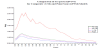
The average values of Sa spectra for 5 random values for different combination of Mw and D (km) are close to each other with the lowest values for Mw= 7.1, D = 10km and the highest one for Mw= 7.8, D = 20km (Figure 15).
3.7 Non-linear soil response analysis of the upper part of soil profiles
Based on above mentioned synthetics it can concluded that
- Closer to near field records are those of M = 7.1 and D = 10km with PGAav = 1.01g for A bridge site and PGAav = 0.98g for L bridge site.
- At the level of input motion (top of Paleozoic rock at ~ 650-700m) the input PGA was determined as 1.0g (for A site and L site).
The upper part with a thickness of 80m is characterized by the nonlinear response of sediments. At depths below the response is elastic one.
- The increase of the thickness of sediments on the top of Paleozoic rocks by 50 meters (L site) has a very small influence on the mean PGA average value (only 0.01g less).
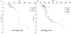
3.7.1 Soil profiles based on shear wave velocity data
The soil profiles of the bridge sites were compiled using geologiclitho logical data and shear wave velocity data from two sources: CH and SASW data.
For L site (Figure 16 a) the SASW testing was performed nearby the location where a seismic cone penetrometer (SCPT) was previously advanced.
For A site (Figure 16b) both SASW and cross-hole data were acquired in addition to the SCPT data at that site.
3.8 Results of Nonlinear Response Analysis for RW and CH Models
3.8.1 Soil Response Profiles
Sa spectra for the shallow soil profile(h~60m) show small differences in the ground response analysis (at periods T = 0.5 - 1.5).
Most of the differences are seen in periods T < 0.5 sec., which tend to be of little significance for bridges and possibly an artificial product of the synthetic motions.
3.8.2 Sa spectra for deep profile
For a deep soil profile the differences in Sa spectra are even less pronounced and comparisons between the SASW and CH data are difficult to identify (Figure 18).
4. Conclusions
For soil profiles modeled using geophysical techniques in NMSZ:
- Equivalent non-linear response analysis for shallow soil model (h~60m) is most pronounced for CH model compared with SASW model. and show small differences in the range T = 0.5 - 1.5sec.
The most differences are seen in the range T < 0.5 sec., which tend to be of little significance for bridges.
- For deep soil profiles (compiled by SASW and CH data ), using the point source model, to generate the synthetics, those differences are even less pronounced and comparisons between the SASW and CH data are difficult to identify.
- Therefore advantages of using high quality CH data for use in ground response are not justified.
- SASW surface geophysics results tend to satisfy the engineering requirements for ground response analysis.
- For shallower deposits and more intrinsic soil-structure interaction analysis the CH geophysical characterization may be justified.
Based on this analysis the main problem in NMSZ is not the high level of amplitudes of strong ground motions, but possible ground failure phenomena to be developed during future strong earthquakes, to be taken into account for the bridges in this area by increasing bearing capacity of the soils and foundations.
Competing Interests
The authors declare that they have no competing interests.
References
- Hoffman D (2003) MoDNR, Geological Survey Program.
- Anderson N, Chen G, Kociu S, Luna R, Malovichko A, et al. (2003) Vertical shear-wave velocity profiles generated from the spectral analysis of surface waves (SASW technique): Field examples from six bridge sites in southeast Missouri. UMR Department of Geology & Geophysics Prepared for MoDOT.
- Kociu S, Luna R, Anderson N, Wei Zh, Hoffman D, et al. (2003) Non-linear response to strong ground motion: Determinations based on SASW velocity profiles. Geophysics, Orlando.
- Khalil MAK (1996) Uncovering Hidden Earthquake Hazards in the Continental United States. The American Physical Society.
- Lillie RJ (1999) Whole Earth Geophysics. Prentice Hall.
- Gutenberg B, Richter CF (1956) Magnitude and energy of earthquakes. Annali di geofisica 9: 1-15. View
- Nuttli O (1973) The Missisipi valley earthquakes of 1811-1812: intensities, ground motion and magnitudes. View
- Street R (1982) A contribution to the documentation of the 1811-1812 Missisipi valley earthquake sequence. Earthquake Notes. View
- Kanamori H, Anderson DL (1975) Theoretical basis of some empirical relations in seismology. BSSA 65:1073-1095. View
- Herrmann RB, Akinci A (1976) Mid-America Ground Motion Models. View
- Boore DB (1996) SMSIM FORTRAN Program for Simulating Ground Motions from Earthquakes: Version 1.0. USGS Open File Report 96-80-A. View
- El-engebawy M (2003) Near-Field Synthetics based on composite model. UMR Dept.of Civil Engineering
- USGS (1996) National Seismic Hazard Mapping Project.
- Zheng W (2003) A computer code built from OPENSES, UMR Dept of Civil Engineering. View
- Gutenberg B, Richter CF (1956) Magnitude and energy of earthquakes. Annali di geofisica 9: 1-15.
- Liu HP, Hu Y, Dorman J, Chang TS, Chiu JM, et al. (1997) Upper Mississippi embayment shallow seismic velocities measured in situ. Engineering Geology 46: 313-330. View
- Ronaldo L, Siasi K, Neil A (2016) Determination of Shear-wave Velocity Profiles from Surface (Rayleigh) Seismic Waves: Wahite Ditch and St. Francis River Bridge Sites, Southeast Missouri.
- NCEER Catalogue of earthquakes of New Madrid and surrounding areas for the period 1795-1995.
- “WESHAKE5” Geotechnical Laboratory, U.S. Army Corps of Engineers Experiment Station. 3909 Halls Ferry Road, Vicksburg, Mississippi. View
- http://quake.ualr/edu/HazardMitigaion/claymitg-plan/Earthquakes.htm View
- http://www.uky.edu/ArtsSciences/Geology/webdogs/virtky/index.html View
- http://www.missouri.edu/~qlpkd/StressEvolution View