1.1 Pseudogenes

A pseudogene is a genomic DNA sequence that is closely related to a gene but has lost the capacity to produce a functional protein. The estimated number of pseudogenes in the human genome is comparable to that of protein coding genes (~20.000) [11,12]. Some pseudogenes are clearly non-functional gene relics [13]. Other pseudogenes, on the contrary, although not translated into proteins, are capable of influencing the activity of other genes by means of long non-coding RNA (lnc RNA) transcripts. In particular, it was observed that some pseudogene transcripts can regulate the expression of their parental genes through competition for cytoplasmic RNA-stabilizing factors or, the other way round, for trans-acting destabilizing factors [14,23]. Moreover, some pseudogenes produce antisense transcripts capable to hybridize with their parental transcripts and leading to suppression of their translation [15].

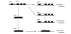
There are three types of pseudogenes. Unitary pseudogenes are formed when spontaneous mutations occur in a coding gene that lead to the loss of either coding or transcription potential (Figure 1A). Unitary pseudogenes are the rarest class of pseudogenes (~100 in humans) [16]. A second class of pseudogenes, the duplicated pseudogenes, is produced by genomic DNA duplication when it is performed incorrectly resulting in a non-functional pseudogene (Figure 1B). A duplicated pseudogene retains the basic structure of functional genes, for example, promoters and introns [17]. The third class, known as the processed pseudogenes, is formed when a mature mRNA is reverse transcribed and integrated into a new location in the host genome (Figure 1C). Because processed pseudogenes are produced from mature mRNA, they usually lack introns and a promoter but, sometimes, they maintain a residue of the RNA polyA tail [18], a stretch of RNA that contains only adenines. In eukaryotes, the presence of a polyA tail at the 3’ extremity is a feature of a mature messenger RNA. Polyadenylation is the addition of a polyA tail to a 3’ messenger RNA. Processed pseudogenes are the most abundant class in humans [12,19] and are formed from just 10% of the coding genes. The type of genes that produce processed pseudogenes are principally highly expressed genes such as genes for ribosomal proteins [19,20].

Figure 1: (A) Unitary pseudogenes, (B) Duplicated pseudogenes, (C) Processed pseudogenes [29].

Pseudogenes are transcribed only if they are integrated close to a pre-existing promoter [12]. Estimates of the number of transcribed pseudogenes suggest that as many as one fifth of the pseudogenes may be transcribed into RNA [12], with processed pseudogenes tending to be transcribed more often than duplicated pseudogenes [21]. Interestingly, several pseudogenes exhibit tissue specific patterns of transcription [18]. Pseudogene RNA levels can also change during differentiation [22] and in diseases such as cancer [23,24] and diabetes [25]. Although pseudogenes are considered to be evolving neutrally, there are many evidences of evolutionary conservation [26,27]. Moreover, pseudogenes with higher levels of evolutionary constraints show greater tendency towards being transcribed [28]. The findings that some pseudogenes have evolved under positive selective pressure and their transcripts can occur in a dynamic and tissue specific manner suggest that they may have an important role.

Characterizing the pseudogenes and understanding their regulatory role is essential to discover the genetic background of many diseases and to identify new pharmacological treatments. Moreover, the correct identification of pseudogenes is important also for gene annotation. Indeed, the prevalence of pseudogenes in mammalian genomes can introduce artifacts in automatic gene annotation pipelines in which pseudogenes are often mistakenly annotated as genes [12,44]. This is due to the high sequence similarity of pseudogenes with their parental genes.

1.2 Aims of the research

Protein sequence similarity to parent gene is the main feature used to detect pseudogenes, because it is deemed the most sensitive indicator [30,31]. In spite of this, we developed a methodology that is based on raw nucleotide identity (DNA sequence similarity) with the coding sequence (CDS) of the corresponding gene and on its transition probabilities. The coding sequence is the portion of the gene that remains in the mature messenger RNA after the splicing and, therefore, it is the portion that is actually translated into protein. It is composed by the exons. Once identified a putative pseudogene, we analyzed both the upstream (before the pseudogene 5’ extreme) and the downstream (beyond the pseudogene 3’ extreme) regions in order to find out biologically interesting features. In particular, we searched for a CpG island and promoter signals in the upstream region. Dinucleotide clusters of CpG, or CpG islands, are present in the promoters and in the exons of ~40% of mammalian genes. However, the abundance of CpG dinucleotides in the human DNA is much lower than expected based on the CG content because CpG dinucleotides, outside the promoters and the exons, are largely methylated. The low occurrence of CpG islands outside these regions is due to the fact that methylated cytosines are mutational hotspots and, as a consequence, they are depleted by natural selection [45,46]. The downstream region, instead, was analyzed in order to detect the presence of a polyA tail and, when a polyA tail was found, a polyadenylation signal was searched for. The polyadenylation signal (typically AAUAAA) is a binding site on the messenger RNA where polyadenylation starts. Moreover, we implemented the Gibbs sampling algorithm with the aim of finding a common motif in the upstream regions containing a CpG island [32,33].

1.3 Main results

In this paper we considered 11 genes and searched for their processed pseudogenes. Five of these genes belong to the ribosomal protein family, which is the family with the highest number of processed pseudogenes [19]. Other six genes are known for their pseudogene mediated expression regulation or for their involvement in cancer disease.

The proposed algorithm was able to detect 110 of 121 pseudogenes annotated by Ensembl for these 11 genes. Moreover, it detected four loci not reported by Ensembl, but reported by UCSC, two new potential pseudogene loci reported neither by Ensembl nor by UCSC and three duplicated sequences for three distinct pseudogenes. Though the algorithm did not capture all the annotated pseudogenes, it seems to be an efficacious solution to detect new potential loci, especially when the query coverage of the alignment is shorter than the coding sequence. These loci can be classified to pseudogene fragments.

The downstream regions of the detected pseudogenes were analyzed in order to find polyA tails. We found a polyA tail for 48 pseudogenes and a polyadenylation signal for 13 of them. These numbers are coherent with known data. Literature reports that a polyA tail is present in about 45-50% of the cases [19].

CpG islands of different lengths and at different distances from the pseudogenes were detected in 16 upstream regions. We didn’t find any motif in the upstream regions probably because a bigger set of sequences is needed by the Gibbs sampling algorithm. However, we executed the algorithm on the flanking regions of some pseudogenes and the results showed an interesting similarity between the flanking regions of some of them. These similarities were confirmed also by alignments of the regions.

1.4 Conclusion and prospects

The complex and not yet elucidated system of interrelations between parental gene mRNAs and pseudogenes transcripts could give reasons for the complexity of vertebrates beyond their genome sizes [29]. Moreover, the comprehension of these mechanisms could bring to light new treatments for many diseases, from cancer to diabetes.

Detection of pseudogenes based on raw nucleotide identity should be applied also for the duplicated pseudogenes. These are longer than processed pseudogenes because they include also introns but, unlike processed pseudogenes, they usually lie in the vicinity of their parental genes and, therefore, their detection does not need the scanning of the entire genome [12].

It was observed that CpG islands not associated with a known promoter (orphan CpG islands) are active transcription initiators during development and, after that, they lose this feature. This evidence suggests that orphan CpG islands are associated with undetected promoters [43]. The search for unknown promoter sequences near the orphan CpG islands in the pseudogenes upstream regions is a promising future development of this work. Moreover, the similarity between the flanking regions of some pseudogenes raises questions about their origin.

2.1 Identification

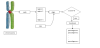
The first step is design of a strategy for identifying the pseudogenes of a gene starting from its CDS. We developed a program that scans the entire genome and stores all the sequences that have similarity with a selected CDS in terms of transition probabilities (the probabilities of transition between the different nucleotides in the CDS) and occurrences of the nucleotides. Each stored sequence is then aligned with the CDS and, if the alignment is statistically significant, the sequence is marked as a pseudogene.

As a first step, the program builds a matrix of the transition probabilities of the CDS and computes the probability of the CDS itself according to this model (CDS_P). The probability is computed as a sum of logarithms of probabilities in order to avoid floating point underflow errors (that is numbers of smaller absolute values than the computer can represent in its CPU) or, worse, the production of arbitrary wrong numbers. The nucleotides occurrences of the CDS $(CD{S}_{C_n})$ are also calculated. A sliding window that has the same length of the CDS scans the entire genome. When it finds a sequence with a transition probability that is included in the interval $CD{S}_P\pm CD{S}_P\cdot 0.05$ and a nucleotide occurrence in the interval $CD{S}_{C_n}\pm CD{S}_{C_n}\cdot 0.2$ , for each nucleotide, the ends of the sequence are stored in a list. The window can enlarge itself until the above-mentioned conditions are satisfied. Sequences longer than four times the CDS length will be discarded from the list at the end of the scanning. A distinct program builds 100.000 random sequences with the same transition probabilities of the CDS. Each sequence is aligned with the CDS and the program returns the mean and the standard deviation of the alignment scores. Then we align the CDS with all the sequences in the list. For each alignment, the main program computes the z-score given by

$Z=\frac{X-\mu }{\sigma },$

using the mean μ and the standard deviation σ previously computed as explained above. A threshold of 8 is chosen for the z-score so that only sequences with a z-score greater than the threshold are recorded as pseudogenes. We chose a threshold of 8 because the alignment scores between the CDSs and the random sequences are not normally distributed [34]. The parameters of the alignment algorithm are: match = 1, mismatch = 0 and gap = -1. Figure 2 summarizes the identification strategy described in this paragraph.

Figure 2: Each chromosome is scanned and the coordinates of all the regions that are homologous to the CDS are stored in the list. Each homologous region is then aligned with the CDS and, if the z-score of the alignment is greater than 8, the region is recorded as a potential pseudogene.

2.2 PolyA tails

A polyA tail is a stretch of RNA that has only adenine bases. In eukaryotes, the addition of a polyA tail to a messenger RNA 3’ end is part of a process that produces mature messenger RNA (mRNA) and is called polyadenylation. Processed pseudogenes are typically characterized by the lack of introns and the presence of residue of the polyA tail, unless it has not decayed [19]. We searched for a polyadenine tail by means of a 50 bp sliding window in the 1000 bp (base pairs) length region beyond the pseudogene 3’ end. The 50 bp windows containing more than 30 adenines are memorized (if they exist) and the most promising one is considered as a PolyA tail. When a polyadenine tail is found, the algorithm searches for a polyadenylation signal (AATAAA or ATTAAA) in the 100 bp length upstream region of the tail.

2.3 CpG islands

CpG islands are regions of DNA in which a cytosine is followed by a guanine in the linear sequence of nucleotides along the 5'→3' direction with a high frequency [48]. The notation CpG is used to distinguish the single strand sequence from the CG pairing on the double strand [49]. In vertebrate genomes, CpG nucleotides occur with a much lower frequency than would be expected by random chance. The frequency of CpG dinucleotides in the human genome is 0.98% while the expected frequency is 4.41%. CpGs cytosines are often methylated (70%). The very low occurrence of CpGs is explained by the fact that methylated cytosines are mutational hotspots and this has led CpGs depletion during evolution [45]. CpG islands usually occur near the transcription start site of genes and have an important role in gene expression regulation. While methylated CpG islands inhibit transcription, unmethylated CpG islands near a transcription start site enables the transcription of that gene. Consequently, CpG islands play an important role in gene expression regulation and the ability to identify them can help us to predict the location of genes within the DNA. A naive approach to locate CpG islands in a sequence X of length L is to extract a sliding window of length $len\ll L$ and to compute a score for each subsequence of length len in X. The main disadvantage of this strategy is that we have no information about the length of the islands. If we use a value of len that is too large, the score we get from this window may not be high enough. The best approach for this problem is the use of a Hidden Markov Model (HMM). A general HMM [35] is a triplet

$M=(Q,S,\Theta ),$

where:

1. Q is an alphabet of symbols;
2. S is a finite set of states capable of emitting symbols from the alphabet Q;
3. $\Theta$ is a set of probabilities, comprised of:
   1. state transition probabilities, denoted as p_{i j} for each i, j $\in$ S;
   2. emission probabilities denoted as q_k(b) for each k $\in$ S and b $\in$ Q.

The HMM for CpG islands has [36]:

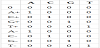
1. 9 states: begin/end, A+, C+, G+, T+, A-, C-, G and T-
2. 4 symbols: A, C, G and T

The letters A+, C+, G+ and T+ represent states that belong to a CpG island. The other letters, instead, represent states not belonging to a CpG island. The state 0 corresponds to the state begin/end of the chain. A Markov chain is a system (S, A) consisting of a finite set of states S and a transition matrix A= a_kl with ${\displaystyle {\sum }_{l\in S}{a}_{kl}}=1$ for all k $\in$ s that determines the probability of the transition k→l by P(s_i+1 =l | s_i =k)= a_kl. At any step i, the Markov chain is in a specific state s_i and the chain changes to state s_i+1 according to the given transition probability [36]. Table 1 reports the emission probability matrix. It’s worth to notice that, in this model, each state emits only the corresponding symbol/ nucleotide (with probability 1).

Table 1: HMM for CpG islands.

The state transition probabilities matrix is reported in Table 2. Model "+" describes the transition probabilities inside the CpG, model "-" describes the transition probabilities outside the CpG island [36].

Table 2: Transition matrix.

The Viterbi algorithm takes as input the query sequence X, the transition probabilities, the emission probabilities of the model and returns a path π that maximizes P(X, π) (may not be unique) [37]. This value is the probability of the most probable path, that is the underlying chain of the HMM. This search performed with HMMs is called decoding and the paths found are called Viterbi paths. Suppose we have a HMM with a finite state S = {G₁,...,G_N} and transition prob abilities $P_{0i},P_{ij},P_{j0}\forall i,j=1,\mathrm{...},N.$ Given a sequence of letters X = X₁... X_L from the alphabet Q, we define

$v_k(1)=p_{0k}{q}_k(X_1)$

for k = 1,...,N. Then we have: $v_k(i)={\max }_{{\pi }_1\mathrm{...}{\pi }_{i-1}}\in X{p}_{0{\pi }_1}{q}_{{\pi }_1}(x_1)p_{{\pi }_1{\pi }_2}{q}_{{\pi }_2}(x_2)\times \mathrm{...}\times p_{{\pi }_{i-1}}{G}_k{q}_k(x_i),$ for i = 2,...,L and k = 1,...,N.

Now we can compute the probability of each step using the initial condition v_k(1) and the following recursive step:

$v_k(i+1)=q_k(X_{i+1}){\max }_{l=1,\mathrm{...},N}(v_l(i)p_{lk}).$

At the end of the execution, we have the probability of the most probable path given by

${\max }_{l=1,\mathrm{...},N}(v_l(L)p_{l0}).$

Since in our model each letter can be emitted by only two states (i+ and i-), we have a simplified version of the algorithm in which, for i = 2,..L, $p_{{\pi }_{i-1}{\pi }_i}=p_{{\pi }_{i-1}{\pi }_{i+}}$ or $p_{{\pi }_{i-1}{\pi }_i}=p_{{\pi }_{i-1}{\pi }_{i-}}$ and q_k(X_i) = 1. To reconstruct the sequence of states, that is the Viterbi path, at each step we form a set V_k(i) made of all integers m for which v_m(i)p_mk = max_l=1,...,N(v_l(i)p_lk). The Viterbi path can be recovered by recursively choosing m_L $\in$ V (L), then m_L-1 $\in$ V_mL (L-1) until m₁ $\in$ V_m2 (1).

2.4 Motif discovery

In order to find potential sequence signals (DNA binding sites or promoters) in the upstream regions in which a CpG island is present, we developed a Gibbs sampling algorithm capable of locating a pattern of subsequences with the highest likelihood. Gibbs sampling is a probabilistic inference algorithm used to generate a sequence of samples from a joint probability distribution of two or more random variables [38]. In bioinformatics, Gibbs sampling is used to detect motif signals in multiple DNA or protein sequences assuming no prior information about the motifs [32,33,39]. Thus, given a set of sequences S=S(1),..,S(n) and an integer w, the algorithm finds, for each sequence S(i), a subsequence of length w, so that the similarity between the n sequences is maximized [39,40]. Let ci j be the number of occurrences of the symbol j $\in$ Σ among the ith position of the n subsequences. Let qij denote the probability of the symbol j to occur at the ith positions of pattern and let pj denote the frequency of the symbol j in all sequences of S. The algorithm maximizes the equation:

$F={\displaystyle \sum _{i=1}^w{\displaystyle \sum _{j\in \Sigma }{c}_{ij}.\log \frac{q_{ij}}{p_j},}}$

where c_{i j} and q_{i j} are computed from the complete alignment of the subsequences. To achieve this result, we designed an algorithm that performs the following iterative procedures:

1. Initialization: randomly chooses a⁽¹⁾,...,a⁽ⁿ⁾, the starting indices of the subsequences in S(1),...,S(n), respectively.
2. Randomly chooses 1 ≤ z ≤ n and computes c_{i j}, q_{i j} and p_j values for the sequences in S\S^(z).
3. According to the model, computes the weights of all possible subsequences of length w in S^(z). The weights are normalized and a new value of a^(z) is randomly selected with a probability proportional to the weights of the subsequences of S^(z). In order to avoid local optima, the starting position with the highest weight is not guaranteed to be chosen. In order to rapidly converge to a solution, the above mentioned random sampling goes on for a fixed amount of time (usually 15 min), then, after the time threshold has expired, only the position with the highest weight is chosen.
4. The algorithm repeats step 2 and 3 until it converges to a fixed pattern of subsequences. The algorithm ends when the same pattern of subsequences is produced for 10 consecutive iterations.

We chose this strategy with the purpose of having many“fast”solutions rather than few“slow”ones.

3.1 Pseudogenes detection

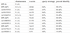
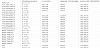
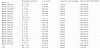
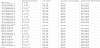
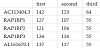
The Ensembl genome browser reports 121 pseudogenes for these 11 genes. We attested 110 of them and we identified 6 pseudogenes loci not previously annotated by the Ensembl genome browser, two of them annotated neither by the Ensembl genome browser nor by the UCSC genome browser (www.genome.ucsc.edu). The statistical significance of the alignments was confirmed by the z-score and by the BLASTN alignment online application hosted by the National Center for Biotechnology Information (NCBI) website (www.ncbi.nlm.nih.gov). The position and the annotation of the sequences found were confirmed by the Ensembl genome browser. Table 3 reports, for each gene, the number of pseudogenes annotated by Ensembl (first row), the number of loci attested by our method (second row) and the loci not reported by Ensembl (third row), but detected by our method.

Table 3: The first row reports the number of annotated pseudogenes for each gene, the second and the third rows report the number of attested pseudogenes and of unannotated pseudogene loci identified by our method respectively.

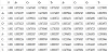
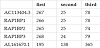
Tables 4, 5, 6 and 7 show the detection results for RPL14, RPL19, RPL22 and RPL37. The first column reports the position in the genome sequence (number of the chromosome, where +1 stands for forward strand and -1 for reverse strand) of the gene itself and of each detected pseudogene. The second column reports the z-score of the alignments. The third and the fourth columns report the query coverage and the percent identity of the alignments respectively. The latter two parameters are provided by BLASTN.

Table 4: The locus AL356967.1 is annotated by Ensembl as “novel pseudogene” residing on chromosome 6 (forward strand) at 104.687.241-104.687.879. UCSC reports it as RPL14 retrogene.

Table 5: The sequence (1) coincides to an intronic sequence of PAK2 (p21 activated kinase 2) on chromosome 3 (forward strand) at 196.823.591-196.824.193. The sequence (2) is aligned by the Ensembl gene browser with the 3’ portion of the novel transcript FP565171.1 on chromosome 10 (forward strand) at 131.895.114-131.895.702. They are both annotated by UCSC as RPL19 retrogenes, but not by Ensembl. Two duplicated sequences, one of AC007683, the other of RPL19P13, were found on chromosomes 7 (forward strand) and 8 (reverse strand) respectively (not shown in the table). Three pseudogenes of RPL19 were not detected (AC092824.1, AC021660.1 and RPL19P1).

Table 6: The sequence (1) is located in an intronic sequence of PHF21A (PHD finger protein 21A) on chromosome 11 (reverse strand) at 46.053.694-46.054.066 and it is annotated by UCSC as RPL22 retrogene, but not by Ensembl. The sequence (2) is located on chromosome 21 (reverse strand) at 41.135.115-41.135.527. This sequence is annotated neither by UCSC nor by Ensembl. We can consider this sequence as a fragment because of its low query coverage in the BLASTN alignment (40%). The algorithm found one duplicated sequence of RPL22P14 on the forward strand of chromosome 6 (not shown). The pseudogene RPL22P17 was not detected.

Table 7: The sequence (1) is located on chromosome 11 (forward strand) at 75.644.799-75.645.091 and it is annotated neither by UCSC nor by Ensembl. Given its low query coverage (45%) and high percent identity (89.63%) in the BLASTN alignment, this locus can be regarded as a pseudogene fragment. The algorithm did not detect AC011753.4 and RPL37P21.

The computation time of pseudogenes detection depends on CDS length because the optimal alignment is computed in O(L²), where L is the length of the sequence. However, the main factor that influences the computation time is the number of homologous sequences found, which is unknown before execution. Table 8 reports the computation time of each experiment.

Table 8: The table shows the length of each CDS and the computation time needed to scan the entire genome in search of its pseudogenes.

3.2 PolyA tails

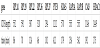
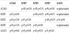
We found 48 polyA tails (41% of the cases) and 13 polyadenylation signals (AATAAA or ATTAAA). It’s worth to notice that the sequence (1) of RPL37, reported neither by Ensembl nor by UCSC, has a polyA tail at 571 bp from its 3’ and a polyadenylation signal at 13 bp from the 5’ of the tail. Table 9 shows the number of tails and the number of polyadenylation signals found for each group of pseudogenes.

Table 9: The first row reports the number of pseudogenes analyzed for each gene (attested+not reported), the second and the third rows report the number of tails and the number of polyadenylation signals for each group respectively.

3.3 CpG islands

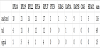
The upstream 1000 bp length regions of the detected pseudogenes were analyzed in order to check the presence of CpG islands. Table 10 displays the number of CpG islands found for each group of pseudogenes and the maximum CpG island length in each group. It is worth to notice that the length of the CpG islands varies a lot and, therefore, a sliding window cannot be used to detect CpG islands.

Table 10: The first row reports the number of pseudogenes analyzed for each gene (attested+not reported), the second row reports the number of CpG islands identified in each group. The last row displays the maximum CpG island length in each group.

3.4 Motif discovery and flanking regions

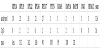
It was observed that half of mammalian CpG islands (~ 10.000) are “orphan”, that is, they are not associated with annotated promoters. There are evidences that many orphan CpG islands play a role as transcriptional initiator during development and, after that, they are subject to DNA methylation loosing their active promoter features. Thus, orphan CpG islands may correspond to undetected promoters that are active during development [43]. With the aim of finding a possible DNA signal in the CpG islands found, we analyzed the 500 bp length pseudogenes upstream regions that contain CpG islands. We run the Gibbs sampling algorithm in order to find common subsequences of length 14. We didn’t find any significant common motif. Nevertheless, we identified a similarity between the upstream regions of RAP1B pseudogenes. We noticed that the subsequences of the best pattern for these regions are located at similar distances from their respective pseudogenes 5’ ends. The same happens for the subsequences of other high-scored patterns. A similar feature was observed also in the downstream regions (excepting AL161670.1). This feature was not observed in the upstream (and downstream) sequences of the pseudogenes of RAP1A, PTEN and HDAC1. We did not test the ribosomal pseudogenes for this feature. Table 11 shows the distances from the 5’ ends of the RAP1B pseudogenes of the three best upstream patterns. Table 12 shows the distances from the 3’ ends of the RAP1B pseudogenes of the three best downstream patterns.

Table 11: The table shows the distances of the three bestscored upstream patterns from the 5’ ends of the pseudogenes of RAP1B.

Table 12: The table shows the distances of the three bestscored downstream patterns from the 3’ ends of the pseudogenes of RAP1B.

A further confirmation of the similarity between the flanking regions of these pseudogenes is provided by the alignment BLASTN online application hosted by the NCBI website. In Table 13, the bottom-left triangle contains the alignments scores (qc = query coverage and pi = percent identity) of the upstream regions. The top-right triangle contains the results of the downstream regions alignments.

Table 13: The table reports the scores of the alignments among the upstream regions (bottom-left) and among the downstream regions (top-right) of the pseudogenes of RAP1B.