1. Introduction

In the field of medical imaging, images of the highest possible quality are essential in order for clinicians to provide the optimal care for their patients. However, in nuclear medical imaging, the image matrix size of the measured results does not change, although restrictions on the image matrix size affect the resulting image accuracy. The primary limitations can be explained as follows. If the total data acquisition time is denoted by T and the total amount of data acquired during this time is denoted by A_(T) , then A_(T) represents the amount of data acquired, C_(t) , per unit time t. This is expressed by the following definite integral (Equation 1) and serves as the foundation of data acquisition in nuclear medicine [1]:

A (T) = ∫ 0 T C (t) dt (1)

If we ignore the half-life and assume no changes in biokinetics, the amount of data obtained over 60 instances of data accumulation in 1s (t=1s, T=60) is the same as that obtained in a single static acquisition in 1 min (t=60s, T=1).

Furthermore, γ-rays produced by radioactive decay are completely random, with no regularity, irrespective of the direction they face and the locations of their incidence points on the gamma camera detectors [1]. If T is divided into n intervals, the count measured during a tiny interval, T/n, is not necessarily constant. In particular, if we focus on the variation in the data acquired during each tiny unit of time, t (t = T/n), a measurement system that obtains 60 counts in an acquisition time of 60 s does not acquire data at a constant count rate for each t, as shown in Figure 1a, but rather records image data as the sum of 60 s of events that occur irregularly, as shown in Figure 1b and Figure 1c.

Figure 1: Relationship between total count and count per unit time (a): The count per unit time is constant; therefore, the total count increases directly with time (b), (c): The count per unit time is random. These are possible events in the real world. Thus, the change in the total count is usually in proportion to time.

In a measurement system that obtains 60 counts in 1 min, if the data variation is observed every second, the integrated value of the data for60 intervals (t = 1 s, T = 60) across a time series (data observed in sequence at acquisition time points 1, 2, 3, …, 60 s) is 60 counts. If an approximation equation across this time series is expressed as y₁ = a₁x + b₁, then y₁ at x = 60 s is extremely close to 60 counts. Because data acquisition occurs in the form of irregular events, the approximation equation y₂ = a₂x + b₂ differs stochastically when the γ-ray acquisition time series is observed in reverse order to the obtained data (at acquisition time points 60, 59, 58, …, 1 s), and although y₁ and y₂ may be very similar values at x = 60 s, normally y₁ and y₂ cannot be equal, because of the irregularity mentioned above.

In other words, even if the data for different 60-s acquisition periods are the same, the values observed during short durations differ, and various approximation equations can be created by rearranging the time series and changing the data observation direction. This indicates that multiple data can be obtained from one time series.

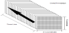
Nearest-neighbor interpolation [2], bicubic interpolation [3], and interpolation by the Lanczos method [4,5] are algorithms for changing the matrix size of an image. In all of these methods, four times the amount of data is normally required to simply double the image matrix size. Complementing the data fourfold from nonexistent data enables twofold enlargement, but problems such as image blurring generally arise [2-5], and various complementary techniques for improving such images exist. However, to the best of our knowledge, no complementary techniques for improving the matrix size in nuclear medical imaging have been reported. Thus, in this paper we examine a filtering method wherein, by observing a time series of the count data in units of t from four directions, four approximation equations are created, and the matrix size is enlarged by complementing it twofold (Figure 2).

Figure 2: Proposed high-resolution image reconstruction method with multidivisional data acquisition. The count-data pattern stored in one matrix (a) shows time series variation. This count-data pattern was arranged in four layouts, from a1 to a4.

Unlike conventional filtering processes [2-8], the present technique effectively enables the improvement of the apparent matrix size while maintaining the quantitative characteristics of the image, without extending the imaging time. In this paper, we describe the capture and analysis of basic data (Experiment 1) and demonstrate a clinical application (Experiment 2).

2. Equipment Used

• Gamma camera: e.cam (Siemens: ICONTM Computer System)
• Collimator: Low-energy high-resolution (LEHR) (Siemens)
• Workstation: ICONP (Siemens)
• Analyzing computing system: PC/AT compatible machine
  • Operating system: Windows XP
  • Software: Borland C++ Builder Ver5.0, Microsoft Visual C++ Ver.6
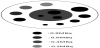
• Phantom 1(Figure3)

  Self-made phantom (99 mTc: 0.2–0.8 MBq administered)

• Phantom 2 (Figure 4)

  Hoffman 3D Brain Phantom TM (99 mTc: 74 MBq administered)

Figure 3: Phantom I: Made in-house using various size cylinders enclosing ^99mTc: 0.2~0.8 MBq.

Figure 4: Phantom II Hoffman 3D Brain Phantom^TM enclosing ^99m Tc: 74 MBq.

3. Experiment 1

When working with the gamma camera, we used phantoms I and II to confirm the variations that were observed in counts within a pixel per unit of time. We also performed reconstruction using the acquired static and SPECT phantom data.

3.2 Analysis method

The image data obtained as described in Section 2-1 were analyzed using a personal computer. Figure5 shows a schematic representation of the data acquisition. The image data used were organized into a data array, Data [Time][x][y], as shown in the figure, and were analyzed across a timeline (time series) for each pixel. That is, data analysis was performed for all pixels by fixing x and y and varying the time from 0 to 60 s in the data array.

Figure 5: Storing image data in time series matrices.

3.3 Image reconstruction

From the static acquisition and SPECT acquisition values, measured at intervals of t = 1 s, a total of four count data patterns were created: (1) the count acquired across the normal timeline, which served as the basic data (Normal)’(2) the data observed in the reverse direction of the timeline (Inverse); (3)the data observed in the positive direction of the timeline beginning at the origin (Forward); and (4) the data observed in the negative time direction (Backward). As an example, Figure 6 illustrates the count data rearranged on the basis of these four patterns using the count data per unit time acquired in the first 10 s. Image data were created by rearranging the data for the set acquisition time into the four patterns, determining a linear approximation equation for each pattern using the least squares method, and replotting the results in a matrix area that was twice as large.

Figure 6: Re-arranged count data classified into four types, namely “Normal,” “Inverse,” “Forward,” and “Backward”, using the count data per unit time of the first 10 acquisitions.

In addition, SPECT reconstruction was performed using simple back-projection without filtering to facilitate comparison of the conventional data acquisition image and the image obtained using the proposed technique.

4. Experiment 2

A Here, cclinical application of the filtering method is wasevaluated, by acquiring static clinical data per unit time, and reconstructing images based on data acquired using the proposed technique.

5. Results of Experiment 1

The actual acquired images and the images reconstructed using the proposed technique are displayed at the same window width and level, to the extent possible.

5.1 Acquisition, analysis, and reconstruction results

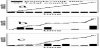
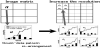
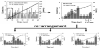
The results of the acquisition, analysis, and reconstruction conducted using the proposed technique are described first, with phantom II as an example. Figures 7 and figure 8 show the variations in count when acquired at intervals of 1 s for 60 s and the resulting variations in the total count. The measurement points are the phantom II image points A, B, and C shown in figure 7, where the vertical axis indicates the acquired count obtained each second and the horizontal axis indicates time. Focusing on the results in the pixel at point C in Figure 8, the average was approximately 2 counts/s, and the total of the count data was 128 counts. The variations in the count data per unit time at points A, B, and C were not constant, but we ascertained that the total count increased with time.

Figure 7: The count-data pattern stores matrices A, B, and C of Phantom II and shows the unit time series variation by acquisition. (Phantom image of 1-s acquisition).

Figure 8: The progress of count in the phantom II acquisition by unit time and the progress of the count sum data for points A, B, and C (shown in Figure 7).

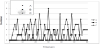
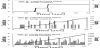
Figure 9 shows the variations in the data obtained by integrating, over1-s intervals, the count acquired for each second on the basis of the data shown in Figure 7. The vertical axis indicates the integrated count data, and the horizontal axis indicates time. When data are acquired for 60 s, the datum that we normally observe is at the endpoint of the graph (60 s on the horizontal axis). When we observed the variations in the data obtained by integrating the count acquired in each second over1-s intervals, certain directionality was observed, and we were able to create approximation equations at each pixel, as shown on the graph. All of the approximation equations presented in this paper had coefficients of determination R²= 0.79 or greater.

Figure 9: Progress of the intigrated acquisition count by unit at time point A, B, and C.(Phantom II) image of 1-s (acqusition).

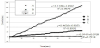
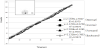
Figure 10 illustrates the results of applying the proposed technique to point C of Figure 7 and Figure 9. Four patterns, namely, (1) Normal, (2) Inverse, (3) Forward, and (4) Backward, were constructed from the time series of acquisitions for a set time, and the data for the approximation equations for four pixels were successfully created using the data for one pixel.

Figure 10: Application of proposed high resolution image reconstruction method to point C (Phantom II images of 1-s acquisition). Approximate expressions of 4 patterns ("Normals," "Inverse," "Forward", and "Backward") computed from 1 pixel count data.

5.2 Phantom I Results

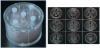
Figure 11(a) shows a static original image of phantom I (128 × 128: 60-s acquisition), Figure 11(b) shows a static reconstructed image (256 × 256) obtained using the proposed technique, and Figure 11(c) shows a static original image (256 × 256: 300-s acquisition). It is understood that the apparent resolution increases when an image is partially enlarged, but this result fell well short of the data for the 256 × 256 matrix that were actually acquired.

Figure 11: Static images of phantom I: (a) Original static image of 128×128 matrix, 60-s acquisition, (b) Reconstructed static image of 256×256 matrix, obtained using the proposed method, (c) Original static image of 256×256 matrix, 300-s acquisition.

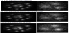
5.3 Phantom II results

Figure 12(a) shows a SPECT original image (128 × 128) of phantom II, while Figure 12(b) shows a SPECT reconstructed image obtained using the proposed technique. The apparent resolution was increased by implementing the proposed technique.

Figure 12: SPECT image of phantom II. (a) Original SPECT image of 128×128 matrix, 60-s acquisition, (b) Reconstructed SPECT image, of 256×256 matrix, obtained using the proposed method.

6. Results of Experiment 2

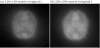
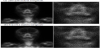
Figure 13(a) shows a clinical static original image (256 × 256: 300-s acquisition), and Figure 13(b) shows a static reconstructed image (512 × 512) obtained using the proposed technique. As in the case illustrated in Fig. 12, the apparent resolution was increased by implementing the proposed technique.

Figure 13: Static image of bone scintigraphy. (a) Original bone static image of 256×256 matrix, 300-s acquisition. (b) Reconstructed bone static image of 512×512 matrix, obtained using the proposed method.

7. Discussion

To double the matrix size of an image, a fourfold increase in imaging time is required when the same statistical elements are used [2-8]. We have proposed a novel filtering method that changes the matrix size without extending the imaging time by making use of the irregularity of the acquisition events. Upon observing the results shown in Figure 11–13, we found that when the proposed technique was implemented using the data acquired in the simple configuration of phantom I, the effect was not as significant as expected. We believe that this is because when the configuration is simple, the effect of the scattered radiation is quite small. Therefore, the γ-rays that reach the collimator are obtained at nearly fixed intervals, and the four approximation equations do not differ significantly [7]. In contrast, in the actual clinical data shown in Figure 13, an apparent effect was observed. Various circumstances affect the creation of nuclear medical images [1], and we believe that statistical variation in the acquisition time has a significant influence.

Variation in the creation of nuclear medical images also depends on clinical factors such as patient condition (which may constrain the possible duration of the examination), dosage, equipment performance, and the nuclide used (specifically, its half-life). If a patient does not remain still during the procedure, data cannot be acquired for the usual set time. The proposed technique can be effective in obtaining the required data in such circumstances. We believe that data acquired with a reduced matrix size and decreased measurement time can be utilized to the maximum degree by applying the proposed technique and that images with increased apparent resolution can be produced. Approximation equations can be created through the proposed technique even with a shorter acquisition time than normal, and by estimating the data for a time interval longer than that of the actual acquired data, an increase in the apparent count can be expected. When this technique is used, images of a higher resolution can be obtained through data acquisition for a shorter time. Further research on this method is currently in progress.

Based on the coefficients of determination obtained in Experiment 1 (R² = 0.79 or greater), we concluded that the reliability of the approximation equations obtained usingthe proposed technique is consistent. However, the shorter the acquisition time is, the lower the reliability is. Further examination of the acquisition time, acquisition process, and approximation method is therefore necessary. Furthermore, in this study, we did not check the degree to which the proposed technique contributed to the actual diagnostic capability. However, it is difficult to imagine that the diagnostic capability would be lower using the proposed technique in situations where diagnosis is possible with currently available nuclear medical image data. The technique described in this paper contributes to an apparent image improvement and unlike typical current filtering techniques that process frequencies in a certain range, the pixel-unit data do not change considerably. This indicates that the quantitative values of the reconstructed data obtained using the proposed techniques do not differ significantly, in a statistical sense, from those collected normally. For the four approximation equations created using the proposed technique, we observed probabilistically similar data within the set acquisition time and obtained the same values when the area of interest was set and average values were determined.

Although the proposed technique requires changes in software for data processing, it is extremely cost-effective because no equipment modification is necessary. In addition, we believe that better-quality images than those possible at present can be obtained through the use of revised techniques and methods for the use of clinical nuclear medicine equipment.

8. Conclusion

The results of this study suggest that an understanding of the variations in time-series data per unit time when acquiring nuclear medicine data makes it possible to produce images with an increased matrix size without extending the imaging time. This can be accomplished by making use of the irregularity of the acquisition events. Although the proposed technique requires changes in software for data processing, it is extremely cost-effective because no equipment modification is necessary.

Competing Interests

The authors have no competing interests with the work presented in this manuscript.

Author Contributions

All the authors substantially contributed to the literature review, drafting the manuscript and approve the final version of the manuscript.

Acknowledgments

We are grateful to Mikio Oishi, Haruo Obara and Shin Maruoka for their constant support and insightful comments.