


1. Introduction
MHD flows involve the motion of an electrically conducting fluid under the effect of an external strong magnetic field and are met in many practical applications such as fusion reactors, electromagnetic pumping and other engineering applications. Thus, different models have been developed for the solution of the Maxwell equations involving different formulations for the induced magnetic field, e.g. [1-7].
The present project involves a geometry with a curved annular duct, as similar geometries are involved in the access ducts of intercooling systems of the dual-coolant breading blankets where lead-lithium (PbLi) is used as the breeder material [8]. Other works involving laminar MHD flows in curved ducts have been performed by Tabeling and Chabrerie [9] at a square channel using an approximate analytical perturbation method and by Issacci et. al [10] in a circular channel with an approximate analytical method. Moresco and Alboussière [11] studied experimentally the instability conditions for the Hartmann layer for the MHD flow on a closed toroidal loop of a square curved duct. The same problem has been studied numerically by Vantieghem and Knaepen [10]. Krasnov et al. [12] studied the problem of linear stability to exponentially growing pertubations in the MHD flow within straight orthogonal ducts. Hoque and Alam [13] studied numerically the MHD flow through a curved pipe of a circular crosssection, under the effect of an axial magnetic field, using a spectral method.
One of the most important issues in the study of the MHD flow is the accurate determination of the induced magnetic field in order the divergence free condition to be satisfied with the highest accuracy. On the previous studies, the divergence of the induced magnetic field was checked to be very small without corrections [14], or it was improved occasionally using numerical or mathematical technicalities [15], without to produce a method for the systematic improvement of the accuracy of the calculation of the induced magnetic field. These problems are related with the fact that the divergence free condition is a first order partial differential equation which cannot incorporates the set of the required boundary conditions in closed space regions. Thus, for the first time in literature, a variational methodology has been developed, which always satisfies the divergence free condition with high accuracy [16,17]. The aforementioned methodology is used in conjunction with the b-formulation which is applied for moderate values of the external magnetic field, taking into account all the components of the induced magnetic field. However, as the external magnetic field is increased to higher values, the h-formulation [18] is preferred, where only the axial component of the induced magnetic field is taking into account, whereas the magnitude of its secondary components is reduced dramatically. In the case of extremely high values of the external magnetic field, the reduced formulation (r-f) is applied where only the axial components of the velocity and the induced magnetic field are taking into account, because either the secondary velocity components become negligible.
2. Problem Formulation
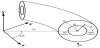
We consider a curved annular duct with radius of curvature Rc and with hydraulic radius R=Ro-Ri, where Ro and Ri are, respectively, the radius of the outer and the inner cylinder, with respect to a Cartesian reference system (x',y',z') of Fig. 1. The liquid metal is subjected to the action of an external magnetic field Bo shown in Figure 1 and the inner and outer cylinders are maintained at uniform temperatures, with the inner wall temperature Ti to be lower than the outlet wall temperature To.
The MHD and thermal flow is governed by the following set of nondimensional equations:
Momentum equation:
Continuity equation:
Energy equation:
Transport of magnetic induction:
Divergence free equation for the magnetic field:
Ohm's law:
Amperes law:
Divergence free equation for the electric current density:
where
The above equations became dimensionless using the following scales
where the prime “ ' ” denotes the dimensional variables, and also
using the following parameters: the Reynolds number
In the assumption of the fully developed laminar forced flow all the
variables
The Cartesian coordinates are transformed to a toroidal-poloidal coordinate system (r,θ,z) using the non-dimensional transformations
where
Introducing the term I=1/(1+κrcosθ), where κ = 1/Rc is the curvature ratio, the governing equations of the fully developed MHD and thermal flow are described below
Continuity equation
Momentum equations at r-direction,
at θ-direction,
and at z-direction
Energy equation
Magnetic field induction equations r-direction
θ-direction
Z-direction
The components of the electric current density are computed from the Ampère’s law
The dimensionless radii of the inner and outer wall are respectively Ro=1 and Ri=0.5. No slip conditions are assumed for the walls, so that u = v = w = 0 for r=Ri and r=Ro. Due to the electrically insulating walls the induced axial magnetic field at the walls with r=Ri and r=Ro is Biz (Ri,θ)=0 and Biz (RR0,θ)=0. The conditions for the boundary conditions for T are To=1 for r=Ro and Ti=0 for r=Ri.
Other quantities of interest are the shear stress at the wall, caused by the liquid metal moving past it, which will be studied using the wall shear stress coefficient and the Nusselt number which is used to study the heat transfer mechanism.
The dimensional shear stress τ'rz and the resultant dimensionless local wall shear stress cf are given by
We define as
The local Nusselt numbers are given for each wall by the following reactions
The average Nusselt numbers for each wall are then given by
3. Computational Methodology
3.1 CVP methodology
The equations (10)-(18) that govern the MHD and thermal flow were solved using a methodology involving the enhanced CVP numerical variational method (Papadopoulos and Hatzikonstantinou, Bakalis and Hatzikonstantinou) for the coupling of the continuity and the Navier-Stokes equation and the coupling of the divergence free condition of the magnetic field with the magnetic field induction equation in the b-formulation. The CVP method characteristics (extreme accuracy, robustness, easy convergence and easy implementation to complex geometries) make it unique for MHD applications.
In this method the partial differential equations are discretized and
solved numerically using a pseudo-transient marching algorithm,
calculating the axial velocity w and the transverse velocity components
The flow is considered fully developed. Therefore, the first and second order axial derivatives are equal to zero except for the axial pressure gradient pa,z. For this case the pressure can be splitted into two terms P=Pa(z)+p(r,θ).
An axisymmetric parabolic profile is used as an initial guess for
the velocity at time level n=1. Then, at each time step an estimation
of the axial velocity w(n+1) and the transverse velocity components
Where
The estimated velocity field does not, in general, satisfy the
continuity equation. Hence, introducing the corrections of the
transverse components of the velocity
The next step is to compute the transverse velocities correction field. From equation (2) we have
Hence, using the irrotational form of the CVP method, at each time
step, the corrections
where
Substituting the transverse velocities (25) into equation (1) at each time level n+1 and by subtracting from this equation (24) we obtain
where
Evaluating the value of
The values of
During the iterative procedure the axial pressure gradient pa,z=∂pa⁄∂z
is considered as uniform over the cross-section and is updated by the
mass conservation equation so that the average axial velocity will be
equal to
Where
3.2 Induced magnetic field formulation (b-formulation)
Using the b-formulation the full set of the MHD equations is solved.
The electric current density is calculated from the Ampere’s law, thus
the divergence free condition for the electric current density is always
satisfied, since it occurs that
A variational procedure is developed consistent with the CVP
methodology in order to ensure that the divergence-free condition of
the magnetic field is satisfied. Solving equations (15)-(17), the induced
magnetic field
Introducing the corrections
From the divergence-free condition we obtain
Using the vector identity
with
Numerical results providing the effectiveness of our methodology are presented in the next paragraph. This methodology can be incorporated with any other computational methodology for the accurate determination of the induced magnetic field in close space regions.
3.3 Computational algorithm and grid
The iterative algorithm begins with an estimation of the velocity and the axial pressure gradient. The velocity components and the pressure are evaluated from the CVP algorithm and with these estimated values the axial component of the induced magnetic field and electric current density are computed using the b-formulation and thereafter the axial pressure gradient is updated. The iteration is repeated until the following convergence criterion for the velocity components is achieved for two sequential time steps,
where
Non-uniform stretched meshes [17,23] are used in order to compute accurately the MHD boundary layers near the walls, and particularly the Hartmann, and side layers, which are respectively vertical and parallel to the magnetic field. Thus, special attention should be paid for the regions near the inner and the outer walls, where thin velocity and electric current layers are formulated due to the effect of the magnetic field, as well as in the right half region of the annulus, where the maximum velocity is formulated due to the effect of the centrifugal and Lorentz forces.
To refine the mesh near the walls, the following transformation for the r-coordinate is used [19]
where
With this formula, a uniform mesh
The following transformation is used in θ-direction twice, in the region between 0 to π and in the region between π to 2π, in order to refine the mesh in the left half region at the left side of the annulus
where sc is the refinement point, τ is the stretching parameter and
The following stretching parameters were used for the relations (34) and (35) are
The effect of the grid on the numerical results for various Hartmann numbers is presented in our work (Bakalis & Hatzikonstantinou, 2015).
4. Result & Discussion
The magnetohydrodynamic and thermal flow of a liquid metal in a curved annular pipe is studied in the present work for Ha=0-2000, Re=100-2000, Gr=0-106, Pr=0.0612, Rm=0.001, and k=0-0.2.
The results are illustrated in order to demonstrate the effect of the curvature and the magnetic field on the velocity distribution. The decrease of curvature κ yields to the decrease of the axial velocity and the reduction of the centrifugal forces. The effect of curvature on MHD flow is presented in our work [18].
The 3D contour plot of Fig. 2 clearly represents the effect of the magnetic field on the axial velocity distribution, for various Hartmann numbers and for Re=2000, Gr=0 and κ=0.2. As it can be observed as the Hartmann number increases side velocity jets are formulated in the left and right regions of the ring-shaped cross section, in a direction parallel to the external magnetic field and the magnitude of the axial velocity w is strongly suppressed at the regions of the Hartmann layers (θ=90° and 270°). These results indicate that as the external magnetic field increases, the liquid metal tends to move mainly by the side regions parallel to the direction of the external magnetic field and tends to be nonmoving at the top and bottom wall regions normal to the external magnetic field.
The suppression of the axial velocity at the regions of the Hartmann
layers (θ=90° and 270°) is presented in Figure 3 with the combination
of the effect of the Grashof number. It can be observed that the axial
velocity profile flattens between the walls and exhibits thin Hartmann
layers near the walls (vertical to
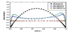
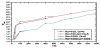
Figure 4 represents the variation of the maximum value of the axial velocity wmax , which appers at angle θ=180°, in terms of the Hartmann number and for Re=100, 1000, Gr=0, 105 and κ=0.2. The peak of the axial velocity increases as the Hartmann number increases, while the effect of the Grashof number is smaller.
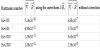
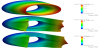
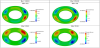
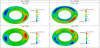
Τhe contour plots of the stream functions of the transverse velocities for various values of the Hartmann and Reynolds numbers are shown for Gr=0 at Figure 5 and for Gr=105 at Figure 6. As the magnetic field increases the transverse components of the velocity are suppressed and two pairs of vortices are redistributed. On the other hand, on Figure 6 it is shown that as the buoyancy forces increase to high values, a stirring of one pair of vortices is presented which increases further as the Reynolds number increases. However, as the Hartmann number increases to higher values, the secondary flow tends to restore the two pair of vortices. For Hartmann numbers greater than 200, the secondary flow is suppressed by orders of magnitude, regardless of the presence of the buoyancy forces.
The stream functions of the transverse components of the velocity are presented in Figure 7 for Re=1000, Gr=105, κ=0.2 and for two different inner diameters (Ri=0.3 and Ri=0.7) than the standard case. It is observed that whereas for the case with inner diameter Ri=0.3 the magnitude of the streamlines is higher than that of Ri=0.5 and for Ri=0.7 is lower than that of Ri=0.5, in both cases, the effect of the external magnetic field highly suppresses the secondary flow and for Ha=200 it has been reduced by one order of magnitude.
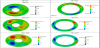
Table 2 represents the effect of the magnetic field and the Reynolds number on the heat transfer as it is expressed by the average Nusselt number on the inner and the outer cylinder, for Grashof number Gr=0 and κ=0.2. It is observed that for small Hartmann numbers, as the Reynolds number increases the average Nusselt number of the inner cylinder decreases and that of the outer cylinder increases, as the secondary flow is shifted to the outer cylinder. Even though, for Hartmann numbers higher than Ha=50 the heat transfer is uniform regardless of the value of the Reynolds number, this is due to the suppression of the secondary flow from the magnetic field.
Table 3 represents the effect of the magnetic field on the average Nusselt numbers, but this time for different values of the Grashof number and for Reynolds number Re=1000. For small Hartmann numbers, under the presence of the Grashof number, the heat transfer on the inner cylinder decreases, while on the outer cylinder it highly increases. This is due to the higher circulation of the secondary flow near the outer wall. For Hartmann numbers higher than Ha=100, the heat transfer is unified, regardless of the presence of the Grashof number or its value, due to the suppression of the secondary flow.
In Figure 8 the contour plot of temperature is presented for various Hartmann and Grashof numbers and for Re=1000 and κ=0.2. It can be observed that the temperature profile is uniform at θ-direction, due to the low value of the Prandtl number. Even though, as the Hartmann number increases from Ha=0 to Ha=50 there is a shift of the temperature profile and an increase of its values. This is due to the increase of the velocity near the outer wall. From Hartmann numbers higher than Ha=50 the temperature profile remains intact.
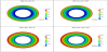
The contour plots of the induced axial magnetic field are presented in Figure 9 for Ha= 10, 200, Gr=0, 105 and κ=0.2. For Ha<100 the induced magnetic field is distributed in two zones parallel to the Hartmann layers. However For Ha>100 the induced magnetic field is distributed into two regions with negative values near θ=45° and θ=135° and two regions with positive values near θ=-45° and θ=- 135°. As the Hartmann number increases the values of the induced magnetic field with and without the effect of the buoyancy forces tend to be equalized due to the suppress of the secondary flow.
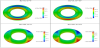
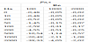
Table 4 represents the effect of the magnetic field and the Reynolds number on the average friction factor of the inner and the outer cylinder for Reynolds number Re=1000 and κ=0.2. As it can be observed, increasing the Hartmann number highly increases the friction factor on both the inner and the outer cylinder, due to the presence of the Hartmann and side layers and the increase of the axial velocity magnitude near the walls.
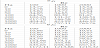
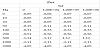
Table 5 represents the variation of the axial pressure gradient pa,z for various values of the Hartmann and Reynolds numbers, for Grashof number Gr=0, and κ=0.2. As the Hartmann number increases the absolute value of the axial pressure gradient highly increases, due to the effect of the opposite direction of the Lorentz force on the direction of the flow.
On the other hand, the effect of the buoyancy forces on the axial pressure gradient is significantly lower as it is presented on Table 6 for Reynolds number Re=1000 and κ=0.2. The impact of the Grashof number on the variation of the axial pressure gradient is significantly small, thus the required pump power on this types of flows can be accurately determined by the effect of the Lorentz force exclusively.
5. Conclusions
The effect of the magnetic field on the velocity distribution of a liquid metal flowing in a curved annular duct with temperature difference between the inner and the outer cylinder is studied in the present work.
From the results it is observed that the axial velocity is slightly affected by the secondary flow which is created by the effect of the centrifugal forces due to the curvature of the duct and the buoyancy forces due to the temperature difference between the inner and the outer wall. It is basically formulated by the magnitude of the external magnetic field, which as it increases formulates two side regions of velocity jets in the left and right half regions of the cylinder and moves the peak of the axial velocity towards the inner wall, while in the regions at the top and the bottom of the annular duct the axial velocity is highly suppressed due to the opposite direction of the Lorentz force. The axial pressure gradient which is required to maintain the same mass flow is significantly increased as the Hartmann number increases, in order to balance the opposite effect of the Lorentz force.
A secondary flow is generated due to the effect curvature of the duct and the temperature difference between the walls. This secondary flow is highly depressed as the magnitude of the external magnetic field increases and becomes negligible for Hartmann values higher than 100~200, regardless of the values of the Reynolds or Grashof number. The curvature and Grashof number were found to have a little impact on the axial pressure gradient in comparison to the effect of the Hartmann number.
Competing Interests
The authors declare that they have no competing interests.