1. Introduction

A central issue emerging during the analysis of time series that measure a property of a given physical system, is what kind of process is generating the observed signal. Linear stochastic processes with infinite degrees of freedom have been used in the past to explain irregular or broadband signals and their Fourier spectrum was believed to be the only tool needed in order to characterize them [1]. On the other hand, nonlinear deterministic processes offer a plausible alternative to linear models for such signals and suggest that a much richer structure may exist in the data. This structure takes the form of fractal geometrical objects, often called strange attractors, that consist of trajectories moving in an m-dimensional Euclidean space (called phase or state space) and represent the evolution of the states of the system under study [2]. Furthermore, a whole new discipline of time series analysis has been established that provides methods to detect and exploit such structure in the data [1,3].

Volcanic tremor is a seismic signal recorded before and during eruptions and is probably related to the subterranean movement of magma and/or venting of gas. On theoretical grounds, volcanic tremor has been identified as being generated by nonlinear processes related to flow of fluids inside volcanic conduits [4,5,6]. Some previous studies have attempted to apply nonlinear dynamics methods to tremor time series recorded at volcanoes around the world, in order to detect the presence of deterministic structure [7,8,9,10]. The main focus of these studies was the reconstruction of the phase space and subsequently either the calculation of the fractal dimension of the resulting attractor, or the detection of temporal changes in the phase space by checking how well the short-term future states of the system are predicted. However, none of the studies mentioned above tried to establish the presence of chaos more rigorously, through a series of tests designed to detect nonlinear dynamics. This is an important point, as it would determine which set of models (linear stochastic or nonlinear chaotic) are more appropriate for describing the tremor source.

The purpose of this study is to investigate the presence of deterministic structure in volcanic tremor time series recorded at Sangay volcano, Ecuador. The selection of the particular dataset for this kind of study is motivated by previous nonlinear time series analysis that had already determined suitable embedding parameters for this tremor data [11]. The paper starts with a summary of the dataset characteristics and of results from previously published studies. Then it proceeds to the description and application of two different tests to the tremor events, followed by the presentation of results and closing with the main conclusions.

2. Data Description

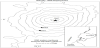
The data used in this study were collected during 21-26 April 1998 and recorded at a sampling interval of 125 "samples per second by two broadband three-component seismometers installed near the active summit vent of Sangay volcano, Ecuador (Figure 1). A spectral analysis of the data published by Johnson and Lees [12] revealed (a) a class of tremor events that are broadband and contain significant energy above 5 Hz, and (b) extended degassing ‘chugging’ events with duration 2-5 minutes that contained well-defined integer overtones (1-5 Hz) and are followed by audible sounds (Figure 2). Events that exhibited high signal-to-noise ratio were selected by Konstantinou and Lin [11] for phase space reconstruction by applying the delay embedding theorem of Takens that uses points y with co-ordinates [1,3]

Figure 1: Topographic map of Sangay also showing as black triangles the locations of the two broadband stations. Inset map shows the location of Sangay in south America (after [12]).

Figure 2: Vertical velocity waveforms recorded at stations near the active vent of Sangay of (a) broadband tremor event and (b) chugging tremor event.

y=s(t),s(t+τ),...,s(t+(m−1)τ) (1)

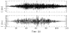
where s(t) are the scalar measurements that compose the seismogram, τ is the delay time and m is the sufficient dimensionfor phase space reconstruction (also known as embedding dimension).

The delay time was estimated after comparing the first minimum of the mutual information and the first zero crossing of the autocorrelation function, while the embedding dimension was determined using the false nearest neighbours algorithm [1,3]. Table 1 gives a summary of these events along with their embedding parameters.

Table 1: Parameters of the tremor events considered in this study after [11].
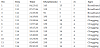
Note: Time is the start time of each event window given in GMT, τ is the delay time and m is the embedding dimension.

3. Surrogate Data Ttest

The term ‘surrogate’ refers to time series having the same linear properties (mean/standard deviation, Fourier spectrum) as the original data, but are otherwise resembling some stochastic process, distorted by the action of a nonlinear static measurement function s_n (similar to linearly filtered noise) given by

s n =s( x n ),  x n = ∑ i=1 M a i s n−i + ∑ i=0 N b i n n−i (2)

where n_n are Gaussian uncorrelated random increments. The time series from such a process can be regarded as linear since the only nonlinearity is contained in the measurement function s. Surrogates can be easily calculated by multiplying the Fourier transform of the data by random phases and then transforming back to the time domain. However, since the same first/second order properties and spectrum with the data cannot be achieved at the same time, an iterative procedure is used in order to minimise any such differences between the surrogates and the data [13].

Once the surrogates are calculated a comparison of a quantity that can be easily estimated from the data against the same quantity estimated from the surrogates is used as a test for detecting deterministic structure. The question of which quantity is more suitable for such a testing has been addressed by Schreiber and Schmitz [14] after performing several tests with time series generated by known chaotic systems (like the tent map or the H´enon equations) and their corresponding surrogates. The authors showed that nonlinear prediction errors performed better in detecting deterministic structure than other tested quantities. Nonlinear prediction errors can be calculated in the following way: assuming that the signal is deterministic, then after reconstructing the phase space the dynamics of the trajectories may be approximated by the difference equation

y n+1 = F(y n ) (3)

where y_n+1 and y_n represent points in the m-dimensional Euclidean space that the phase space lies. Knowing the present state of the system y_n it is possible to predict one step into the future y_n'+1; since the function F describing the evolution of the dynamics is continuous, a past state y_n' very close to the present one is taken and its image y_n+1 is used as the predicted value. Because all interpoint distances are contaminated with an uncertainty due to the finite resolution of the data, all points in the phase space closer than a distance r are equally good for predicting y_n+1. By forming a neighborhood u(†) of radius r around y_n, the final predicted value will be the arithmetic mean of all the images yy_n'+1. The nonlinear prediction error can then be defined as [13,14]

γ= ∑ [ y n+1 −( 1 | u (†) | ∑ y n'+1 ] ) ] 2 (4)

where |u(†)| is the number of points inside the neighborhood u(†). Since the primary assumption of the method described above is that the signal is deterministic, its application to a time series generated by a linear process with no structure in the phase space (like the surrogates), is expected to yield a larger value for γ.

The surrogate statistical test is posed as the formulation of a null hypothesis that states that the data are generated by the process described by equation 1. This hypothesis can be rejected only in the case when the data have a smaller nonlinear prediction error than their corresponding surrogates. The level of significance of this rejection is given by (1 − α)×100%, where α is the probability of a false rejection [13]. Then the number of surrogates that have to be generated as a function of α is 1/ α − 1. If we aim for a significance level of 95% (α = 0.05), then 19 surrogates have to be generated for each tremor event tested. This test is only suitable for broadband tremor, as the null hypothesis assumes that the time series is linearly filtered noise; on the contrary, chugging events have a strong periodic component which is incompatible with this null hypothesis.

The delay times and embedding dimensions listed in Table 1 were used and the initial neighbourhood size for making predictions was set to the interval of the samples in the time series divided by 1000. A minimum number of 30 neighbours was required in order to predict one step into the future. If the neighbours found were less than the minimum number, the neighbourhood size increased by a factor of 1.2 until enough neighbours could be found. For all of the broadband events tested we found that the null hypothesis could not be rejected at a 95% significance level, since they exhibited a slightly higher prediction error than the surrogates (Figure 3). According to Schreiber and Schmitz [13] such a negative result may have two possible interpretations: (a) the process generating the data is a linear stochastic one and the null hypothesis is true, or (b) the prediction error quantity may not be able to detect any structure, possibly because the tremor time series cover at this sampling rate only a fraction of the nonlinear dynamics.

Figure 3: Results of the application of the surrogate data test to the four broadband events considered in this study. The long spike in each diagram represents the original data, while the short one each of the 19 surrogates.

4. Casdagli’s Test

Another method to perform short-term nonlinear predictions is to try to approximate the function F that describes the evolution of the trajectories in the phase space (equation 2) by fitting a simple linear function to a part of the trajectory inside a neighbourhood u(†) of radius r. In this way a predicted value (one step into the future) y ^ n+1 will be given by [3]

y ^ n+1 = a n y n + b n

the coefficients of the model a_n and b_n can then be easily calculated by minimizing in a least-squares sense the difference between actual and predicted values:

σ 2 = ∑ ( y n+1 − a n y n − b n ) 2 (6)

Casdagli [15] suggested that locally linear models can be used for testing data for the presence of deterministic structure. If the prediction error is lower at large neighbourhood sizes, the data are in this embedding dimension best described by a linear stochastic process. On the other hand, low prediction errors at small neighbourhood sizes support the idea of the existence of a nonlinear, almost deterministic equation of motion. Casdagli’s test is much more general in its assumptions, therefore it can be applied to broadband as well as chugging tremor events.

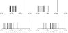
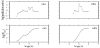
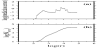
The test is first applied to the broadband tremor events and their surrogates using the same embedding parameters (τ, m) as in Table 1 and predicting one step into the future. For consistency with the surrogate data test, we chose the neighbourhood radius r to range from a minimum value equal to the interval of the data divided by 1000, to a maximum value equal to the interval of the data increasing it each time by a factor of 1.2. Figure 4 shows plots of the prediction error curves for the tremor events and their surrogates while also plotted is the distribution of the number of neighbours found for different r values in each case. It can be seen that the curves corresponding to tremor events show a trend of reduced prediction errors as the neighbourhood size is decreasing, which is absent in the surrogate data curves. The application of this test to the chugging tremor events shows very similar results to the broadband ones, with reduced errors in smaller length scales (Figure 5). These observations seem therefore to support the suggestion of the presence of determinism in the Sangay tremor data. In the next section an explanation is given for this apparent conflict of results between t 2 2 he surrogate and Casdagli tests.

Figure 4: Results of the application of the Casdagli test: (a) logarithm of the prediction error versus the logarithm of the length scale r of the data for a broadband event; (b) the same for one of its surrogates; (c) logarithm of the average number of neighbours N_ave found at length scales r versus log r for the same broadband event; (d) the same for its surrogate.

Figure 5: Same as in Figure 3 (a)-(c) for a chugging event.

5. Conclusions

Despite the fact that theoretical models and many observations lend support to the idea that volcanic tremor should be a low-dimensional chaotic phenomenon, there are many difficulties involved when trying to provide concrete evidence about it. The correlation dimension [16] has been used in the past as ‘indicator’ of determinism, even though it is quite susceptible to the presence of small amounts of noise and heavily depends on the quantity of the available data [1,3]. Thus, any interpretation of a possible scaling region that does not extend through a range of length scales can be considered either as uncertain or as ambiguous. Surrogate data tests were designed so as to remove in theory this ambiguity, however, they also rely on the calculation of some quantity from the data that will be compared later to the value of the same quantity calculated from the surrogates.

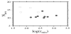
The conflicting results of the surrogate data and the Casdagli tests for the volcanic tremor time series presented in this study, can be explained on the basis of the number of points that are available in different neighbourhood sizes. For the tremor events under study, the number of neighbours in the smallest length scale is between 13-16 (Figure 6). This means that at this smallest length scale the number of available neighbours in order to perform a prediction for the surrogate data test, is smaller than the minimum number set in section 3 (30 neighbours). The algorithm therefore will enlarge the neighbourhood size by a factor of 1.2 in order to find at least 30 neighbours. Unfortunately, this is achieved at neighbourhood sizes that yield prediction errors similar to or larger than the ones calculated from the surrogate data, leading to the acceptance of the null hypothesis.

Figure 6: Diagram showing the average number of neighbours (N_ave) at the smallest length scale of the data (r_min) versus the log r_min. The open circles indicate the broadband events, while the filled ones the chugging events.

At this point it should be noted that the size of the neighbourhood or the number of neighbours needed in order to make a reliable prediction is in most cases not known a priori. In fact the value of 30 neighbors used by the prediction algorithm in the surrogate data test can be considered as a reasonable choice for many dynamical systems [18]. Another solution would be of course to lower the minimum number of neighbours (e.g. to 10), but this may result in compromising the accuracy of the prediction. It appears therefore, that only an adequate number of neighbors at small length scales can ensure the reliability of the results of the surrogate data test. The paucity of neighbors at these scales may indicate that the process generating the tremor signals has been to some extent undersampled. There is evidence that such undersampling may result in an increase of the dimensionality in some signals [17], however, its exact effects on the nonlinear dynamics of volcanic tremor time series are not known and should be investigated in future studies. The results obtained here also highlight the need for reassessing the way seismological data are acquired. The common practice nowadays is to set the sampling interval to 100 samples per second which is even lower than the one used in Sangay. It is clear however, based on the results of Chouet and Shaw [4] that 200 samples per second is the minimum needed for obtaining higher resolution orbits in the phase space and unambiguous estimates of correlation dimension. This is likely to result in more accurate modeling of the source process of volcanic tremor.

Competing Interests

The author declare that there is no competing interests regarding the publication of this article.

Acknowledgments

I would like to thank the Ministry of Science and Technology of Taiwan (MOST) for the financial support of this research. The TISEAN package [18] was used for estimating prediction errors and for surrogate data generation. I would also like to thank an anonymous reviewer for his constructive comments.