


1. Introduction
The use of innovative technologies summarized as Precision Agriculture (PA) is a promising approach to optimize agricultural production of crops. In crop production, precision agriculture methodologies are applied for the site-specific application of fertilizer or pesticides, automatic guidance of agricultural vehicles, product traceability, on-farm research and management of production systems. Precision agriculture can be described as information technology applied to agriculture. Farmers have always known that certain parts of a field produce differently than others, but until precision agriculture came along, farmers lacked the technology to apply this knowledge. The basis of precision agriculture is that it allows the study of fields on a much finer resolution. This in turn provides opportunities for higher yields and lower costs. Farm producers may have the opportunity to optimize production outputs with the application of technologies of precision agriculture.
This new farming management concept is based on observing, measuring and responding to inter and intra-field variability in crops. Crop variability typically has both a spatial and temporal component which makes statistical/computational treatments quite involved. It is only through the adoption of GPS (Global Positioning System) control that this has become possible for farmers. GPS has given farmers the ability to locate their precise position in a field which allows them to measure and record geo-referenced information. This information can then be used in the future to influence management decisions.
Thus, advances in machinery that include the ability to accumulate detailed crop production data and advances in analytical tools to distill these data into performance metrics are changing the way these businesses are managed. For many years, farmers have benefited from the use of yield monitoring data in making management decisions. Since the late 1980s, technology for yield monitoring and accurate positioning has been available with the expansion of application since the early 1990s. The basis of precision agriculture is the opportunity yield monitoring affords in the provision of spatially detailed information in management when coupled with appropriate methods and analysis. One could simply say this is essentially the application of information technology to agriculture.
Consequently, taking into account the relevance of the applications of the modern computer science technologies in the agricultural context, we decided to develop a mobile unmanned terrestrial vehicle (UTV) aimed at assisting the crop monitoring [1,2]. The remainder of the paper is organized as follows: section 2 describes the most relevant related works in the current literature in the context of the agricultural technologies. Section 3 discusses the materials and the methods used, while section 4 presents the experimental method. Finally, some preliminary experimental results are shown in section 5 and conclusions with possible future work are provided in section 6.
2. Related work
In agriculture, knowledge of the characteristics of plants is essential to perform an efficient and effective management of crops. In recent years, the availability of affordable sensors and electronic systems capable of facilitating the performance of intensive measurements has gradually replaced traditional methods based on manual measurements. Currently, there is hardly any relevant plant characteristic without an associated sensory system based on the use of electronics for its determination.
As a result, the accuracy of the measurements has drastically increased; data acquisition has been eased, lightened and, in many cases, automated. Thus, the traditional analysis of a reduced number of manually-collected data has given way to the processing of files with huge amounts of data resulting from the measurements provided by the sensors and decision making in crop management can be supported by information now available and impossible to have in the past. Among the characteristics of crops, geometry deserves special mention (canopy height, width and volume) as well as structural parameters (leaf area index, canopy porosity and permeability and wood structure) due to their great influence on the behavior of plants interacting with solar radiation, water a d nutrients at their disposal Lee and Ehsani [3] as well as on the knowledge and prediction of the vigor and quality of the produced crop. These parameters also have a key role in assessing the efficiency and effectiveness of the main operations performed in the orchards, such as the application of inputs (fertilizers, irrigation and plant protection products against pests and diseases), pruning and harvesting [4,5]. Several studies have shown the existence of a relationship between the geometrical parameters of a crop and yield. Among the geometric parameters of plants, canopy volume has a special significance because it combines, in a single variable, the width, the height, the geometric shape and the structure of trees [6]. For this reason, its determination in a reliable, systematic and affordable way, both in cost and time, is a priority in the present and near future of Precision Agriculture/ Fructiculture defined as the one that takes full advantage of the ICT (Information and Communications Technology) systems, geostatistics and decision making support systems. Usually, precise measurement of the volume of a canopy requires of costly man-made measurements on the plants with the corresponding time and economical cost. However, several sensor-based approaches have been published in the scientific literature dealing with the problem of estimating the canopy volume. The techniques used to determine the canopy volumes are based either on the use of electromagnetic radiation, mainly in the spectrum range from the ultraviolet to the infrared, including the visible, or on the use of ultrasonic waves. The most widespread systems in the first group are those based on the use of digital photography, photogrammetric, and stereoscopy techniques as well as LiDAR (Light Detection and Ranging) sensors [5]. A LiDAR sensor estimates the distance apart of the object of interest, using in some technologies the Time of Flight (ToF) principle [7]. In practice most used LiDAR scanners perform sweeps in a plane (2D) or in the space (3D) by modifying the direction at which the laser beam is emitted. A very common configuration in agricultural research applications is what is known as mobile terrestrial laser scanner (MTLS), a 2D LiDAR sensor mounted on a vehicle moving along the alley-ways between rows of trees in an orchard in order to obtain the scanning of the entire crop in 3D, [8]. This operation mode usually requires a high precision GNSS receiver to know the spatial coordinates of the LiDAR sensor at all times.
In Keightley and Bawden [9] a LiDAR sensor mounted on a ground tripod is used for 3D volumetric modeling of a grapevine. The system does not consider position errors and the validations were performed under laboratory conditions. In Bucksch and Fleck [10] and in Raumonen et al. [11] a ground fixed LiDAR sensor is used to 3D model the tree skeletons, based on a graph splitting procedure to extract branches from the cloud of points. Although the system efficiently extracts the skeleton patterns from several trees, it does not offer a real time solution and its robustness to leaves density is not provided in the research. In the same line, Cote et al. [12], explores and tests the use of LiDAR scanners in tree modeling. In addition, Moorthy et al. [13] used 3D LiDAR to measure structural and biophysical information of individual trees. Fieber et al. [14] used a LiDAR to classify ground, trees and oranges using only the reflected waveforms from the LiDAR, avoiding the need of using geometric information. Although efficient, the proposal was not tested for real time implementations but for batch processing only. In addition, no information is provided regarding shapes or sizes of the agricultural features. In Walklate et al. [15] a LiDAR sensor and a GPS receiver are mounted on a same chassis for 3D reconstruction of orchards. No information is provided regarding the geometric processing. Instead, the research is focused on using the 3D information for spray management. The performance of the previous methods relies on the precision of the GPS (see Auat Cheein and Guivant, [16]. Mendez et al. [17] used a LiDAR for skeleton reconstruction of a grove and for vegetative measures.
On the other hand, Jaeger-Hansen et al. [18] uses a similar hardware and provides a first estimate of the treetop surface using ellipses and minimum square fitting techniques.
In addition, in Rosell et al. [19], a first study in 3D orchard reconstruction is presented, in which a LiDAR and a differential GPS are used for mapping the environment. Moreover, optical crop-sensing technology has been around for several years [20,21]. Optical cropsensing systems use light sensors to analyze in-season plant health. Healthy plants absorb more red lights, and less healthy plants take in less. Optical crop-sensing systems are currently available mostly through Trimble with Green Seeker and AgLeader with OptRx. Both systems measure crop status and variably apply the crop’s nitrogen requirements in anhydrous, dry or liquid form. While both optical crop-sensing systems generally work the same, there are differences. Green Seeker calculates Normalized Difference Vegetative Index (NDVI), a way to measure plant health [22]. The NDVI is an indicator of biomass living plant tissue and is combined with known growingdegree days to project yield potential [23,24].
To help determine the correct nitrogen recommendations and application rates, Green Seeker calibrates using a nitrogenrich strip which is really a control base. The strip is used to establish a midseason determination of additional nitrogen requirements. The strip must be present in each field and should be 300 to 500 feet long, and in a representative area of the field. It should not be in the upland or bottom area, but should have different soil types or topography.
OptRx utilizes a virtual reference strip instead of a nitrogen rich strip for making nitrogen recommendations [25]. Much like Green Seeker, the OptRx system assigns a vegetation index value based on plant biomass and nitrogen content. Thus, the OptRx crop sensor uses a single algorithm to control application.
3. Materials and Methods
We have developed a crop monitoring mobile unmanned terrestrial vehicle based on a combined use of optical sensors aimed to assist our preliminary tests.
3.1 The mobile lab
The main materials used to develop the overall system are a set of co-operating sensors. More in details, we used 2 Lidar sensors and 3 OptRx crop sensors, which are described in SubSections III-B and III-D. Moreover, a sonar sensor, in order to have a better indication of the position of the mobile lab, in terms of distance from a movable target (e.g., a vertical panel) and a RTK GPS are installed on the system.
The real time kinematic GPS (RTK GPS), provides GPS position accuracy to within 1 centimeter. RTK GPS requires a separate base station located within approximately 5 miles of the mobile GPS units. Thus, the RTK base station is a known location equipped with a GPS unit. The base station GPS location is corrected to its known location, and the correction factor is transmitted to the mobile GPS units by FM radio signals. The accuracy of RTK GPS results from the close proximity of the base correction station. However, the data acquisition phase is essential for our whole process. Thus, the data captured from the sensors in our system are in the order of millions (for instance 6.5 GBs when considering a one-hectare field), we plan to define and exploit in the future some specific indices in order to significantly improve the data analysis efficiency. For example, we can use a customized implementation of the tMAGIC [26] (Temporal Multiactivity Graph Index Creation) index, that first stores into a huge log (called temporal multiactivity graph) the multiple activities that need to be concurrently monitored and then defines an efficient algorithm to find the activity that best matches a sequence of observations. This index has been already efficiently exploited by other relevant works, such as [27-30].
We also plan to carry out two different types of experiments:
- A very accurate but less representative reconstruction just of a small subset of the overall data set. We will be working at a very low speed on small plots (5 m). The total disk consumption would be around 3.25 MBs.
- A less accurate but very representative reconstruction of the overall plot (one hectare). We will be using a low sampling frequency and working at very high speeds (4km/h). The total disk consumption would be around 6.5 GBs.
3.2 Lidar Sensor
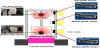
In this experimental work the two LIDAR scanners used were a general-purpose SICK LMS-111 model (Sick 1, Du sseldorf, Germany) (Figure 1), with a range accuracy of 30 mm, a selectable angular resolution of 0.5 degrees and a scanning angle of 270 degree. Moreover, the LMS-111 has a standard RS232 serial port for data transfer and an ethernet port.
The software tools used along with the two LIDAR sensors are SOPAS ET 1.0.4, to complete the customized configuration of the LIDAR device, Hercules Setup Utility 3.2.8, to manage the communication with the sensor and the data transmission, and Matlab, to make a detailed analysis on the data obtained during the previous steps. When the laser beam is intercepted by the surface of vegetation, the sensor determines from the reflected signal the angular position q and the radial distance r between the target interception point and LIDAR position. The sensor continuously measures distances at the selected angular resolution.
This information represented a vertical outline (or slice) of the tree for the current position of the LIDAR. When moved along the rows, the LIDAR scanner supplied a cluster or cloud of plant interception points in polar coordinates (r,q). Although the LMS-111 LIDAR is a 2D laser scanner, the displacement of the laser sensor along the direction (Z) parallel to the row of trees at a known constant speed, and the use of software allowed a 3D graphic representation of the cloud of plants interception points to be developed, such that a nondestructive record of the tree-row structure of the crop was obtained. Once the 3D cloud of points was obtained, efforts were focused on obtaining the geometrical and structural parameters of the tree and bush crops under examination.
3.3 The developed LIDAR/NDVI algorithm
Considering the following input/output parameters:
- X1: higher-level lidar coordinate.
- X2: lower-level lidar coordinate.
- tol: tolerance defined by the user.
- X: X coordinate value,
The developed LIDAR/NDVI algorithm is defined as follows (Algorithm 1).
| Algorithm 1 LIDAR/NDVI algorithm |
| Input: LIDAR data, NDVI data, tol |
| Output: X |
| 1: Extraction of the cylindrical coordinates. |
| 2: Conversion into cartesian coordinates. |
| 3: Mesh generation along Z and Y of size d (defined by the user (d=0.01 m)) and interpolation of the Lidar data for the X coordinate. |
| 4: Merging the both side Lidar data. |
| 5: Merging data algorithm on the base of tol. |
| 6: X = X coordinate evaluation(X1;X2; tol) (see Algorithm 2). |
| 7: Mesh generation along Z and Y with the same size d as Lidar and NDVI data interpolation. |
3.4 OptRx Crop Sensor
Available from AgLeader, the three OptRx Crop Sensors used in our work2 are able to record and measure real time information.
| Algorithm 2 X coordinate evaluation |
| Input: X1, X2, tol |
| Output: X |
| 1: if |X1- X2| < tol then |
| 2: X = (X1 + X2) / 2 |
| 3: else |
| 4: if X2> X1 then |
| 5: X = X2 |
| 6: else |
| 7: X = X1 |
| 8: Return X |
OptRx crop sensors work by shining light on the crop canopy and reading the light reflected back to determine the crop health, also known as Vegetative Index. Moreover, the Vegetative Index (VI) aquired are NDVI (Normalized Difference Vegetation Index) and NDRE (Normalized Difference Red Edge Index) with a scanning angle of 45 - 10 degrees and a measurement range of 0.25-2 m. The normalized difference vegetation index (NDVI) is historically one of the first VIs. It is a normalized ratio of the NIR (near infrared) and red bands [31].
NDV I = (NIR - Red)=(NIR + Red)
Theoretically, NDVI values range from +1.0 to -1.0. Areas of barren rock, sand, or snow usually show very low NDVI values (for example, 0.1 or less). Sparse vegetation such as shrubs and grasslands or senescing crops may result in moderate NDVI values (approximately 0.2 to 0.5). High NDVI values (approximately 0.6 to 0.9) correspond to dense vegetation such as that found in temperate and tropical forests or crops at their peak growth stage.
Moreover, the Normalized Difference Red Edge [32] uses the NDVI form but substitutes its bands by a red edge band at 720 nm and a reference band from the NIR plateau at 790 nm. Since OptRx uses its own light sensing technology, there is no dependence upon ambient light or angle of the sun [33]. OptRx can be used day or night when optimum conditions are available. Data collected is logged and mapped into a device, which automatically records application activities, including applied areas, product volume, and more. After that, using the proprietary AgLeader Software SMS basic, the different information can be easily downloaded into AgLeader SMS software for analysis. Consequently, using this information and also managing it, we were able to use the 3D-Field Software to process the optical measurement in order to obtain the NDVI maps which immediately show differences in vegetative development among plant groups.
3.5 The overall system
- Unmanned Terrestrial Vehicle (UTV)
- two LIDAR sensors
- tree NDVI crop sensors
- one Sonar range finder
Measurements were made using the UTV which supports our six sensors and traverses the experimental crop in direction Z, parallel to the row at a known and costant speed; the crop used for such experiments are described in the following section. More specifically, the LIDAR sensors were placed on our UTV at two different heights (0.544 and 1.531 m), vertically aligned and scanning the same targets; furthermore, the OptRX sensors were also put on the UTV at three different heights (0.59, 1.088, 1.587 m), still vertically alligned and scanning the same targets (Figure 1 and 2).
Moreover, the progress speed has been estimated through sonar managed by the Arduino board that was mounted on the overall system as well. The sensor measures distances, that are considered as instantaneous as well as the sample speed. The average constant progress speed has been chosen as reference speed value. This speed was 0.3-0.5 m/s for both sensors.
4. Experimental Method
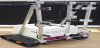
The Unmanned Terrestrial Vehicle (UTV) developed was used to characterize some common trees (Figure 3). The species analyzed are the following:
- Cupressocyparis Leylandii Spiral, height 160 cm
- Cupressocyparis Leylandii Ball, height 140 cm
- Cupressocyparis Leylandii Pon Pon, height 160 cm
- Juniperus virginiana, height 240 cm
- Pachira, height 110 cm
- Ficus benjamina, height 160 cm
The trees were aligned in a chain from left to the right, in the order listed above. Then, a fake plant whose layout is obviously well-known is added to the top (i.e., left) of this plant line. Furthermore, some reference panels [34] were placed as shown in Figure 3. Thus, an experimental activity aimed at acquiring data in different scenarios related to a decreasing distance between the plants - from a maximum of 1 meter to a minimum close to 0 - was performed.
5. Results and Discussion
Following the experimental method previously explained, we obtained some very promising results. The main innovations of this case study are the combined use of Lidar and NDVI sensors to get real time information about both the geometric shapes and the vegetative states of the plants, and the canapy reconstruction of our plant line, using the path shown in Figure 3.
For the first of the reasons listed above, the data obtained with the Lidar and NDVI elaborations have been processed using Matlab, in order to discover the correspondences of these point clouds and their correct over lapping. The scan performed by the LIDAR sensors (Figure 4) meshed with the OptRx ones (Figure 5) showed some really interesting results. From the exhibited diagrams, we can notice how the NDVI maps reconstruct the vegetative state of the plant line of interest.
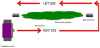
The LIDAR + NDVI diagram in (Figure 6) was plotted in order to discover the X coordinate of the plant midpoint. The obtained X coordinate of the plant midpoint is x0 = 1.85 m. Then, we exploited such a value to compute the vegetative thickness (d) as follows:
Right side: d = x0 - x
Right side: d = x - x0
Where x is still the X Lidar coordinate
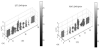
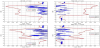
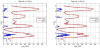
Then, we chose 4 different height (y) values (respectively, 0.6 m, 1.0 m, 1.4 m and 1.8 m), and plotted on the same diagram:
- The vegetative thickness on the X axis and the Z coordinate on the Y axis
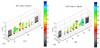
- The NDVI index on the X axis and the Z coordinate on the Y axis both for the left and for the right sides, as depicted in the following diagrams Figure 7.
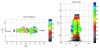
On the other hand, the following diagrams Figure 8 & 9 were plotted still taking as reference the same height values, but considering some 20 cm slots along the Y axis, then computing the average of both the thickness and NDVI. Moreover, in the following diagrams (Figure 10, 11), we can notice a change in the NDVI index trend in correspondence to a high thickness value. Differently from the previous diagrams, in the following ones we used some 10 cm slots along the Y axis.
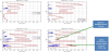
Another area where the NDVI index is low can be found in correspondence to the sphere shaped plant trunk, obviously because there is no vegetation.
Furthermore, a 40 cm slot as a whole was used, 20 with reference to the height of interest.
Eventually, the diagrams below (Figure 12) were plotted to compare the curve trends when fixing the height value (y) to 0.6 m and using a different slot size; at left 20, while at right 10. In the right one, we can notice a more marked change in the NDVI trend.
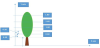
For the second one, the tractor completed a path while scanning both the sides of the plant line analyzed. From this scan we derived the following diagram (Figure 6) showing an excellent volume reconstruction of the plant line in both the scanned sides. As a matter of fact, as depicted in Figure 13, the reconstructed plants are very similar to their real geometric shapes.
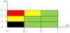
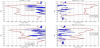
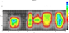
Eventually, the two reconstructions have been meshed in order to obtain the overall line volume reconstruction. In order to improve the visual representation of the vigour map, we have implemented a novel diagnostic algorithm based on the matrix of Figure 14. The matrix rows discretize the vegetation thickness in three different ranges:
- t ≺ 0.1m
- 0.1 ≺ t ≺ 0.2m
- t ≻ 0.2m
While the matrix columns discretize the NDVI index in three different ranges:
- NDVI ≺ 0:6
- 0.6 ≺ NDVI ≺0:8
- NDVI ≺ 0:8
As a result, the black element of the matrix represents an area without vegetation. The yellow elements describe a critical situation, while the red ones correspond to a very critical vegetation area. Eventually, the green elements outline the healthy vegetation. According to Figure 14, this novel diagnostic algorithm highlights a better different vegetation health status in comparison with the NDVI representation of Figure 10. Plants B and E are healthy. Plant D has a vigour region, while has also some unhealthy regions where foliage is sparse in the bottom part of the trunk. Plant C has a critical region because the NDVI sensor captured the woody zone in the middle of the sphere. Finally, plant A is overall healthy, but it shows a much stressed area (the unhealthy leaf marked in red).
The novel diagnosis algorithm showed an excellent potential in this preliminary investigation stage. In order to correctly illustrate the health condition of the plants, a refinement of this algorithm will be carried out in the future experiments to find out the optimal range of vegetation thickness and the NDVI vegetation index to be applied to the diagnosis matrix.
Finally, the LIDAR (Light Detection and Ranging) sensor technology installed on the unmanned terrestrial vehicle (UTV) is equipped with a rotating mirror mechanism, which deflects the laser beam emitted. With such a mechanism the LIDAR allows for time measurements not just of a point, but of a 2D slice of the environment. In case of bad weather conditions (rain or snow) a laser pulse can be reflected by a raindrop or a snowflake preventing from measuring the object of interest.
In order to improve the LIDAR performance in bad weather conditions, a multi-echo technology was introduced. When a laser pulse is emitted, the energy propagates through the environment in a cone shape, as not all of it will typically be reflected by a rain drop or snow flake. However, it must be keep in mind that the mobile lab was conceived to detect crops under normal weather conditions, in order to avoid any type of undesired interference with the measuring system. Furthermore, the NDVI sensors can operate autonomously, emitting pulse light.
6. Conclusion
Recent trends in global agriculture prices have brought a new scenario for agricultural policies worldwide. Increased world demand for agricultural products combined with interannual fluctuations of global production mostly caused by climate variability have been an important cause for price volatility in agricultural markets, and social unrest in many parts of the world. In this context, crop monitoring and yield forecasting play a major role in anticipating supply anomalies, thus allowing well-informed timely policy action and market adjustment, preventing food crises and market disruptions, reducing market speculation, and contributing to overall increased food security.
Moreover, we plan to define and exploit in the future some specific indices in order to significantly improve the data analysis efficiency, potentially combined with the management of multimedia data depicting, for instance, the plant evolution over time [35].
Future work will exploit the NDVI index, calculated from reflectances in the red and near-infrared (NIR) portions of the spectrum, rather than other indices such as EVI. The EVI index incorporates reflectance in the blue portion of the spectrum in addition to the red and NIR. Moreover, one of the biggest current limitations to implement EVI is that it needs a blue band to be calculated. Not only does this limit the sensors that EVI can be applied to (e.g., ASTER has no blue band), but the blue band typically has a low signal-to-noise ratio. In addition, further future experiments will be devoted to discover the optimal slot sizes on which to average the thickness and the NDVI index, in order to obtain a better representation and an automated statistical method will be defined in the next future to both identify best predictors and indices.
The solution here developed clearly focuses on orchard applications, as it applies proximal sensing detections able to provide lateralviews of the canopy, instead of top-views typically provided by conventional remote sensing surveys carried out by flying vectors. Future improvements are still expected in merit to aspects such as: the capability to estimate the thinning intensity according to the bloom charge, early diagnosis of diseases, and detection of nutritional stresses.
However, we also plan to use our mobile lab in a wide range of agricultural contexts, including arable crops. To this aim, some minor modifications will be provided to the sensor supports in order to be able to get typical top-views to acquire information on the physiological state of the herbaceous crops.
Acknowledgments
The research leading to these results has been supported by the Monalisa project, which was funded by the Autonomous Province of Bozen-Bolzano.