1. Introduction

The building energy used for HVAC is about 49% of the total energy consumption of commercial buildings in Korea [1].There have been many studies on energy saving efforts in buildings including the development of efficient systems and renewable energy sources as well as the implementation of smart system operation strategies. Air-to-air heat exchangers have been used to recover exhaust energy [2-4] and various ventilation control strategies have been proposed for HVAC systems [5-10]. Demand-controlled ventilation (DCV) is an energy saving approach for regulating the amount of outdoor air supplied to a building based on demand. It is important to choose appropriate control parameters reflecting the demand for ventilation adequately. The control parameters include the concentrations of various indoor contaminants and the strengths of contaminant sources. It is difficult to reflect the room demand for ventilation based on a single control parameter out of many contaminant concentrations. Carbon dioxide concentration has been widely selected to be used for ventilation control, since it represents the degree of overall indoor pollution [11,12]. However, CO₂ concentration level does not represent the demand for ventilation based on heat, moisture, and dust generated from occupants or occupant behavior in general. To consider several parameters at once, a complex sensor network and a high-performance computer are required. While occupants are beneficiaries of good indoor air quality, they also are sources of various effluents including carbon dioxide, particulate matters, heat, and moisture. Provisional approach is provided by specifying minimum ventilation rate for each person [13]. Therefore, the number of occupants in a space can be a meaningful control parameter for DCV.

There are several ways to count occupancy, such as installing infrared motion sensors, image sensing by deciphering the shadows in a photo, and smart sensing with RFID sensors. However, these methods are inadequate for occupancy measurements in public facilities. Because a large number of people may move simultaneously within a large space, motion or image sensing has some uncertainties [14,15]. RFID sensing requires a high-performance system and heavy costs. Moreover, some of the aforementioned methods may have some privacy issues. Another method of obtaining occupancy information is to infer the information from other parameters.

A subway is a commonly used public transportation system in metropolitan areas such as Seoul. There are about three-hundred subway stations in Seoul, and 80% are located underground [16]. It is difficult to naturally ventilate an underground space. The indoor air quality can deteriorate greatly when subway stations are crowded, such as during rush hour. Mechanical ventilation consumes a lot of energy when the ventilation requirement is large, such as in a subway station. Energy saving in a subway station requires an appropriate control method, and DCV based on occupancy can be a suitable candidate. In this study, we use a method that estimates the occupancy based on the CO₂ concentration on a subway platform. The CO₂ generation rate by humans is difficult to measure exactly because it depends on the amount and type of activity; in addition, the natural ventilation rate is also difficult to measure exactly. We therefore use a statistical method, i.e., Bayesian inference, to consider these uncertainties.

2. Subway Station Modeling

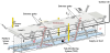
The station under consideration is an underground subway station in the 4^th line of Seoul metropolitan area. This station is one of the most crowded stations in Seoul. There are approximately 17 million passengers annually on the average. The station has two underground levels. The first level is the concourse level, where there are offices, waiting zones, and entrance gates to the platforms. The second level has two different types of spaces: a platform from which the passengers get on and off the trains, and a tunnel through which the trains operate. Platforms are located symmetrically on both sides of the two-way rail track. The platform spaces are separated from the rail track space by platform screen doors (PSDs) installed for safety. Each platform is 200 m long, 2.5 m high and 6.4 m wide on one side. The length corresponds to the length of a train with ten passenger cars. The platform volume is shown with the dotted lines in Figure 1.

Figure 1: Layout of the underground subway station.

Mechanical ventilation fans normally operate 24 hours a day with a constant outdoor airflow rate. The numbers of passengers entering and leaving the platform are counted at entrance and exit gates separately. The numbers are summed up on an hourly basis at both the entrance and exit gates. A Tele-Monitoring System (TMS) has been installed in the station to continuously monitor the indoor and outdoor environmental conditions, including the temperature, humidity, CO₂, PM₁₀, and NO₂ concentrations. The system is for indoor monitoring purposes, but not for ventilation control purposes. In this study, TMS data acquired on October 7, 2010 were used, which were taken at every 5 minutes.

The platform area and the train tunnel can be treated as independent compartmental zones since the installed PSDs are of a complete-seal type. The platform zone is the control volume under consideration for the present study. The air in the control volume is assumed to be fully mixed, and thus the concentration is uniform throughout the volume. The air change rate of the control volume is determined using a mechanical ventilation system. The air leakage through the PSDs is neglected, as is the air exchange through the stairways between the platform on the second level and the concourse on the first level.

Carbon dioxide concentration at the platform is determined by the CO₂ mass balance equation shown in Equation (1) with the aforementioned assumptions. The solution can be expressed as in Equation (2).

V dC(t) dt =Q[ C ∞ −C(t) ]+N m ˙ (1)

c(t)= N m ˙ Q +[ c o − N m ˙ Q ] e − Q V t (2)

Where V is the air volume in the platform, and Q is the ventilation rate. The capital letter C is the absolute concentration whereas c is the indoor concentration subtracted from the background concentration c = C - C_∞). In addition, N is the number of passengers present in the control volume, and is the CO₂ generation rate per person.

3. Bayesian Simulation

Bayesian method estimates the posterior probability as a consequence of a prior probability and a likelihood function derived from a probability model for the data to be observed [17]. Bayesian inference computes the posterior probability according to the Bayes’ theorem. Bayes’ theorem for probability can be extended to determine the probability variable and its distribution function. An extended theorem is used to generate the posterior distribution through a combination of the prior distribution and likelihood. An extended theorem can be expressed as in Equation (3).

π( θ|x )= π( θ )f( x|θ ) ∫ π( θ )f( x|θ )dθ (3)

where π (θ) is the prior probability of θ assumed and f(x|θ) is the likelihood of observing x given θ. π (θ |x) is the posterior probability of θ obtained after x is observed.

A simple static Bayesian model is based on the steady-state concentration, C ¯   = N m ˙ /Q , which can be obtained from Equation (2) easily. Assuming both the generation rate and the ventilation rate remain constant, the space concentration is proportional to the number of occupants in the space. Therefore, the number of occupants can be determined by only the current concentration level but not by the concentrations at previous steps.

c Δt =(1−α) c ¯ +α c o (4)

The concentration at the next time step, c_Δt ,is the weighted average of the steady concentration,c , and the concentration at the previous time step, c_o. The weighting factor, i.e. α = exp (-QΔt/V), depends on the time interval, Δt. For a large time interval, the weighting factor is close to zero, so that the concentration at the next time step is mostly determined by the steady concentration but not by the previous concentration. For a short time interval, however, the previous concentration plays a more important role than the steady concentration in determining the concentration at the next time step.

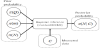
The prior information that should be inputted include the ventilation rate, Q, the CO₂ generation rate per person, m, and the number of occupants, N. The variables involved in Bayesian inference are shown in Figure 2. The nominal ventilationcapacityof the station is known to be 4,000 m³/h. The actual ventilation rate can vary depending on the weather conditions, such as outdoor temperature and wind speed. It is assumed conservatively that the mean is the nominal capacity and the standard deviation is 30% of the mean. The metabolic generation rate of CO₂ varies from one person to another, depending on the activity level of the person. It is also assumed to follow a Gaussian distribution, with the mean of 18 L/h [13], and the deviation of 30% of the mean. Of all the given conditions, occupancy is the variable in which the prior information is the most uncertain, and can have any value from zero to infinity. Both Gaussian and Poisson distributions were tested for the prior probability distribution of occupancy. The static model calculates the steady concentration based on the distributions of the prior probability of the input variables, such as the ventilation rate, generation rate, and occupancy. The dynamic model calculates the current concentration using Equation (4), based on the distributions of the prior probability. The samples are accepted when the criterion is exceeded by the obtained post-probability as compared with the measured concentration data during the time step. The uncertainty in the CO₂ measurement is assumed to be 5% of the reading. The occupancy is inferred at every 5 minute interval. A total of 10,000 calculations are repeated at each time step.

Figure 2: Concept of a Bayesian inference.

Program ‘R’ was used for Markov Chain Monte Carlo (MCMC) simulation. The program includes various statistical and numerical analysis modules, and is useful for analyzing data for a statistical inference [18]. Figure 3 shows a flowchart of an MCMC simulation. We used the Metropolis-Hastings method to extract a sample of the posterior distribution. The first step is to input the prior information. As mentioned earlier, the prior information is the mean and standard deviation of the ventilation rate, the CO₂ generation rate per person, and the occupancy. The next step is to generate the prior distribution based on the prior information. This distribution is used to calculate the probability of the proposed values of Q,m, and N . Each proposed value is generated randomly from the proposed distribution based on a jumping parameter. A jumping parameter is made up of the standard deviations of Q,m, and N and is assumed empirically. We used 10% of the mean for all jumping parameters. In sequence, the proposed CO₂ concentration is calculated based on the proposed values of Q,m and N, and the likelihood of the proposed CO₂ concentration is calculated from the distribution of the measured CO₂ concentration. This likelihood is compared with the likelihood of the previous iteration, and the likelihood ratio is used to accept or reject a sample.

Figure 3: Flow chart of the algorithm used in theMCMC simulation.

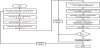
Figure 4 shows a typical variation of CO₂ concentration in a platform measured on a weekday. Starting at midnight, the concentration decreases slowly during the night, and increases quickly after the first train starts operating in the morning. During the morning rush hour, the concentration rises up to 1,000 ppm. After 11:00, the concentration remains nearly constant throughout midday. There is an evening peak between 18:00 and 21:00, which is lower and wider than the morning peak. After the evening peak, the concentration drops slowly to an ambient concentration until the next morning.

Figure 4: CO₂ concentration measured on the platform, and the numbers of passengers counted at the entrance and exit gates.

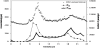
The exact number of persons present in the platform is very difficult to measure on a real time basis because the floating population is large and varies continuously. The actual occupancy is derived from the number counts at the gates. The numbers of people entering (n_out ) and leaving (n_enter) the platform hourly are shown in Figure 4. The entering number count is the sum of passengers passing through all entrance gates, and the exiting number count is the sum through all exit gates. Even though the two number counts differ from one another at a given time step, their daily sums are equal. The actual occupancy is calculated by considering the train service interval and the escape time for passengers to leave the platform [19]. Table 1 shows the hourly mean and standard deviation of the train service interval.

Table 1: Hourly mean and standard deviation of train operation interval.

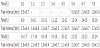
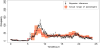
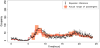
Figure 5 shows the results of the Bayesian inference obtained through the static model using a Gaussian distribution for the prior probability distribution. The occupancy was inferred at each time step with 5 minute intervals. The black dots are the mean values of the MCMC samples, and the bars across the dots indicate the ranges between the lower 10% and upper 90% of the selected samples. The daily pattern of the inferred number of occupants shows a pattern similar to that of the measured concentration data. The inferred ranges fall mostly within the estimated ranges based on the actual passenger numbers counted at the gates, which is shown with shaded areain red. Note that the inferred values are somewhat delayed in time.

Figure 5: Results of the Bayesian inference by the static model.

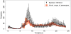
The dynamic model needs to be used to consider the time delay in the concentration responses after a change in the source strength. Figure 6 shows the results of the dynamic model, which considers the concentration differential in addition to the current concentration value. Note that the time step is 1 h, and the time constant based on the air exchange rate is approximately 1.25 h. It can be observed that the vertical bars showing the inferred ranges are reduced significantly, and that the errors are also lowered. In particular, the inferred occupancy is closer to the actual occupancy especially during 19:00- 23:00 than the static model.

Figure 6: Results of the Bayesian inference by the dynamic model.

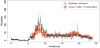
Figure 7 compares the errors by the static and dynamic models. The errors are the hourly means of the instantaneous errors between the actual and estimated values. The errors by the dynamic model are much smaller in 8:00-10:00 and 19:00-23:00 when the concentration fluctuates considerably, but are greater in 11:00 to 18:00 compared to those by the static model. The error bars are not shown between 2:00 and 4:00, because the actual occupancy during this period is zero. The dynamic model gives more or less uniform error ranges, whereas the static model gives large variations in the error ranges based on the time of day. The average error per day for the static and dynamic models is 40±41% and 27±25%, respectively.

Figure 7: Comparison of errors from the static and dynamic models.

When the prior information is unknown for a positive variable other than its mean value, the Poisson distribution is preferred. In the Gaussian distribution, the variable can be negative in case the standard deviation is assumed to be large compared to the mean value. In the Poisson distribution, only positive values are considered, and negative values are not extracted.

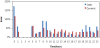
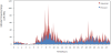
Figure 8 shows the simulation results of the dynamic model using the Poisson distribution. As before, the black dots indicate the mean values of the selected samples, and the bars indicate the lower 10% to the upper 90%. The mean values are nearly the same as those obtained using the Gaussian distribution, but the inference ranges were significantly reduced. This result can be seen clearly in Figure 9, which shows the degree of error bars of the MCMC samples with both the Gaussian and Poisson distributions. The Gaussian and Poisson distributions have a range of 7.6±7 and 13.5±14 on average, respectively.

Figure 8: Results of the Bayesian inference using a Poisson distribution.

Figure 9: Comparison of the range in Gaussian and Poisson distributions.

However, the errors during the morning rush hour are relatively large because the CO₂ generation rate per person is assumed to be constant throughout the day. During the rush hour, however, the passengers are considered to be relatively active and young, and hence their metabolic rates are relatively high. In contrast, the movement of passengers during midday is relatively slow, and the generation rate may be lower than during the rush hour. The age distribution of passengers is not discussed further in detail since it is beyond the scope of the present paper. The occupancy is over-estimated during the morning rush hour, and under-estimated during the midday, because the present analysis does not include the generation rate based on the time of day.

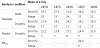
Table 2 shows a summary of the aforementioned results during the entire experimental period. An error is the percent ratio with the actual occupancy, and the range is the gap in the error band of the estimation. The errors and ranges of the dynamic model are smaller than the results of the static model for all days. For the Poisson distribution, the errors are similar to those of the dynamic model, but the ranges are a little bit smaller. This result shows that the dynamic model improves the accuracy, and the Poisson distribution improves the degree of precision. The last row in the table shows the results for when the PM₁₀ data are used along with the CO₂ data to improve the accuracy.

Table 2: Summary of Bayesian inference results during weekdays.

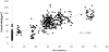
Particulate matter is a typical indoor contaminant that has recently come to light. The human body and clothing are direct sources of particulate matter, and human movement can increase the particle concentration by reviving the dust settled on a floor surface. The relationship between PM₁₀ concentration and occupancy in a space has yet to be verified, but the possibility has been suggested in several studies [20,21]. Figure 10 shows the correlation between PM₁₀ concentration and the estimated occupancy on the platform. The coefficient of the correlation is 0.63, and the PM₁₀ concentration can be related to the occupancy of the space. As mentioned earlier, we use the PM₁₀ concentration as an additional parameter to improve the accuracy of the estimation. The MCMC samples obtained from the CO₂ data were again input into a Bayesian loop based on the PM₁₀ correlation to obtain filtered MCMC samples. Figure 11 shows the results on Oct. 7. The error is decreased remarkably between 8:00 and 9:00, and the inferred occupancy is close to the actual occupancy between 9:00 and 11:00.

Figure 10: Correlation between PM₁₀ concentration and actual occupancy.

Figure 11: Results of the Bayesian inference using the PM₁₀ concentration.

4. Conclusion

A feasibility study has been conducted to investigate the possibility of using the current IAQ monitoring system for demand controlled ventilation in a subway station. The number of occupants in the platform was estimated based on CO₂ concentration data using the Bayesian inference. The mean values and uncertainty ranges were inferred statistically by the calculation models, both static and dynamic, of the CO₂ concentration, as well as the prior Gaussian and Poisson distributions of occupancy. The results were compared with the actual occupancy derived from the number counted at the gates. The following conclusions have been drawn.

1. The Bayesian inference method provides reasonable estimates of occupancy in a subway station even though various assumptions should be made for prior probabilities.
2. An appropriate physical model is required in order to use the CO₂ concentration as the parameter for occupancy estimation. The dynamic model results in less uncertainty than the static model by implementing the time delay in the concentration responses after a step change in the source strength.
3. For the prior assumption of occupancy, the Poisson distribution is preferred, since it requires a single input parameter and does not result in negative values. As a result, the Poisson distribution creates a smaller inference range than the Gaussian distribution.

The uncertainty has been reduced by applying additional PM₁₀ concentration data to the MCMC samples based on the CO₂ concentration data to obtain filtered samples. We cannot conclude that this method is optimized, since the relationship between PM₁₀ concentration and the occupancy of the space has not been fully verified. However, we can conclude the PM₁₀ concentration can used as an additional parameter for improving the accuracy of the present method.

A proper ventilation model should be used to improve the accuracy in the application of the presented Bayesian method, and the proper probability distributions should be used to improve the precision. Further studies should be conducted to improve the applicability ofthe Bayesian method using various models for different applications.

Competing Interests

The authors declare that they have no competing interests.

Acknowledgments

All the authors gratefully acknowledge the supports. We thank Seoul metro for providing information on system operation data, and Korea Environment Corporation for providing indoor air quality data taken from Tele Monitoring System.