


1. Introduction
Surficial geological mapping is traditionally based on the interpretation of aerial photographs using a stereoscope and then ground-truthed byfield work. However in Arctic regions, field surveys are time-consuming and costly because of the remote access and the lack of infrastructure for logistical support of field programs. To address these limitations and assist in the interpretation of the surficial geology, an improved method for mapping surficial materials is the use of satellite imagery in concert with digital image processing techniques. This approach offers the advantages of extensive regional coverage, no aerial or ground disturbance of the areas to be mapped, as well as complete and cost-effective data coverage. Optical images such as Landsat or SPOT can be used [1], but optical images cannot be acquired at night or during cloudy conditions. These limitations do not exist with synthetic aperture radar (SAR) images, such as those acquired by RADARSAT-2 [2,3], because SAR is an active sensor that generates its own microwave energy and therefore image acquisition is independent of atmospheric conditions. However, image quality can be affected by ground moisture related to weather and climate.
Previous research of using Synthetic Apeture Radar (SAR) imagery for mapping surficial materials of northern Canada was limited largely to single frequency and single polarization sensors on board of RADARSAT-1 [4-6]. More recent studies have employed the advantages of multi-polarized SAR images, particularly the combination of like- and cross- polarized data [3,7,8]. Crosspolarized images can measure depolarization over areas of vegetation [9] and extreme surface roughness [10]. Combining SAR and optical imagery offers several advantages because both image types are complementary [5-7,3,8]. SAR images are sensitive to surface texture by providing information on scattering mechanisms that are related to surface roughness and moisture content [11,3]. Optical images are sensitive to surficial reflective properties that are generally governed by surface chemistry, vegetation, and surface moisture content [12].
This research is part of a surficial geology mapping effort under Natural Resources Canada’s Geo-mapping for Energy and Minerals (GEM-1 and GEM-2) programs to provide new geological knowledge on the nature and composition of surficial materials for sustainable resource development and land-use management in central mainland Nunavut [13-16]. The study is subdivided into two parts: part 1 [8] produced a surficial materials map with 21 classes for an area located north of Wager Bay by applying a non-parametric supervised classifier (Random Forests) to a combination of Landsat 8 optical images and RADARSAT-2 SAR C-HH and C-HV images as well as a digital elevation model (DEM) and derived slope data; part 2 applies the same methodology developed and validated in the area north of Wager bay to produce a surficial materials map comprising 22 classes for an area located south of Wager Bay, Nunavut. The resultant map is validated with an independent set of georeferenced field observations that were acquired in summers of 2012, 2015, and 2016.
2. Study Area
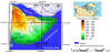
The study area is located south of Wager Bay, Nunavut, on the western side of Hudson Bay and includes parts of Ukkusiksalik National Park (Figure 1). It covers the National Topographic System (NTS) map sheets 046D, 046E, 055P, 056A, 056H. The study area is located within the Wager Plateau of the Canadian Shield [17]. Elevations range from sea level along Wager Bay and Hudson Bay to 550 m asl in the northwestern part of the study area. The drainage network lianks numerous intermediate to large lakes and ponds (Figure 1). The overall discharge direction of drainage systems is from west to east through Roes Welcome Sound into the Hudson Bay, or south to north for the uplands that slope abruptly into Wager Bay (Figure 1). The climatic conditions in the study area are of an arctic climate. The vegetation is typical of the Arctic tundra and is mainly composed of dwarf shrubs, birch, willow mixed with herbs, lichens, and mosses [18]. Soils in the lowland areas are thin organic soils (peat), whereas other soils are cryosols associated with deep permafrost (frozen soil) and related periglacial landforms [18]. However, the active layer thaws during the summer months, and creates standing water and/or saturated soils, which may interfere with radar backscatter [3].
The geomorphology of the region is characterized by streamlined terrain which extends southeast from a former major ice divide zone (Keewatin Ice Divide), from which ice flowed radially during the last glaciation [13]. The Keewatin Ice Divide was centred in the uplands southwest of Wager Bay and its eastern extremity extended in the study area over NTS 56H and 46E map sheets, forming a landscape now dominated at surface by till of varying thickness, felsenmeer, and weathered bedrock [13,15,16,19]. This glacial landscape is interspersed by a complex system of subglacial meltwater corridors and proglacial meltwater channels. The subglacial corridors comprise large eskers, small irregular hummocks, and ridges of sandy diamicton, short streamlined landforms of till, boulder lags, washed bedrock surfaces, and outwash plains. In former proglacial meltwater systems, till surfaces show extensive erosion and/or reworking. The limit of postglacial marine submergence ranges from 113m above mean sea level (AMSL) south of Wager Bay to about 152m AMSL west of Roes Welcome Sound [19]. Lowlands that skirt the coasts of Roes Welcome Sound show evidence of postglacial marine erosion and reworking of thin glacial and glaciofluvial sediments [15,16]. Glaciomarine veneers are sandy and occur as scattered deposits between rock ridges or glacial landforms. Preliminary surficial geology maps compiled at the 1:100,000 scale as part of the GEM program in NTS 46D and 56A prior to field work [20-22] are based largely on air-photo interpretation with minimal ground-truthing. In NTS 56H-south, Randour and McMartin [23] more recently compiled a surficial geology map based on detailed field observations. Frost-riven, rough and lichen-covered outcrops occur sporadically across the area, and are mainly concentrated in meltwater corridors, in coastal lowlands along Rose Welcome sound or in the uplands south of Wager Bay; glacially polished bedrock outcrops are rare and more common along the coast in the intertidal zone.
3. Data Sources
Five Landsat-8 images were acquired by the Operational Land Imager (OLI) sensor over two years from 2013 to 2014 (Table 1). These images were mosaicked together to cover the entire study area. They were visually checked to ensure that the ground was free of ice and snow and did not include any clouds or shadows. The Landsat 8 images were already georeferenced in a NAD83 format (UTM Zone 16, Row W) and have eight bands: B1 (0.43-0.45 μm), B2 (0.45-0.51 μm), B3 (0.53-0.59 μm), B4 (0.64-0.67 μm), B5 (0.85-0.88 μm), B6 (1.57-1.65 μm), B7 (2.11-2.29 μm), and B8 (0.50-0.68 μm).
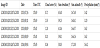
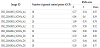
Eight RADARSAT-2 Scan SAR Wide-A C-band dual-polarized (HH and HV) images acquired during August of 2014 were used for this study (Table 2),with an incidence angle increasing from 20 and 49.3° from the center to the image corner. Four SAR images were acquired with an ascending orbit resulting in an east-looking direction and four with a descending orbit resulting in a west-looking direction (Table 2). While the ascending orbit images were acquired during dry conditions, the descending orbit images were acquired during dry and wet conditions, as Byatt [24] showed that the accuracy of surficial material maps increases when optical and SAR images acquired over dry and wet conditions are combined. Each image file had two images: the HH polarized image and the HV polarized intensity image. All the images were checked visually to ensure the ground was free of snow and ice cover.

Ancillary data used in this study included several 1:50,000 digital elevation model (DEM) tiles [25], that were downloaded from GeoGratis database [25]. The DEM has a resolution of 16.1 m in the x direction, 23.3 m in the y direction and 1 m in the z direction. Ground elevations are recorded in meters relative to mean sea level (MSL), based on the NAD83 horizontal reference datum. The DEM tiles were used for terrain correction when georeferencing the SAR images and for correcting the topographic effects in the Landsat mosaicking process. The DEM was also used to compute the slope. Both the DEM and slope were used as input features in the classifier.
Two types of georeferenced sites were used in the study. The first one consists offield observations collected at 45 sites during the summer of 2015 as part of a GEM-2 funded project [26,15]. They consist of ground pictures, Ground Position Satellite (GPS) coordinates, and detailed descriptions of the surficial materials. The second type of GPS sites were determined from photo-interpretation of helicopter-based pictures collected in 2015 and of Google Earth images [27]. About 648 GPS sites were used to validate the produced map. Another510sites were used to delineate training polygons of at least 10 pixels for a total of 2216 points. Both the training and validation GPS sites were distributed across the study area (Figure 2). Details on the distribution of the training and validation GPS sites within the surficial material classes are presented in the Image classification section.
4. Methods
4.1 Image processing
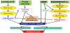
The flowchart shown in Figure 3 provides a summary of the image processing methodology used in the study. The majority of the image processing was performed in PCI Geomatica 2015® software. The DEM tiles were first imported and then mosaicked together using the Ortho Engine module of PCI Geomatica 2015®. The resulting mosaic was also used to compute a slope mosaic. The digital numbers of the Landsat 8 OLI images were first converted into top of atmosphere (TOA) reflectance values, following the method described in the Landsat 8 users handbook [28]. This conversion also removes some of the atmospheric interferences.
Following methods utilized by Grunsky et al. [5] and LaRocque et al. [3], the RADARSAT-2 C-HH and C-HV images were filtered to help suppress the effects of speckle using a Gaussian filter (with a standard deviation of 1.6). Speckle is a multiplicative noise and its intensity must be attenuated in order to enhance fine details on SAR images [29]. Each individual image was then orthorectified with the “RADARSAT-2 Rational Function Model” function provided by the Orthoengine module of PCI Geomatica 2015®, using the DEM and ground control points (GCPs). Approximately 20 GCPs were extracted from the orthorectified Landsat 8 data for georeferencing, achieved with a mean accuracy of less than one pixel in both x and y axes (Table 3). The georeferenced images were then mosaicked together to cover the entire study area. This was accomplished using the OrthoEngine module of PCI Geomatica 2015®, using the "Automatic Mosaicking" menu that requires the use of the DEM. The parameters used in the mosaicking method were as follows: histogram for the full image, adaptive filter: 20 % of the image, match area: 10 %, cutline: minimum difference, and blend width: 20 pixels.
4.2 Image classification
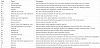
The same surficial material classes were used as was utilized for the Wager Bay North area [8], with some exceptions (Table 4). A specific surface materials class used in the Wager Bay North study, carbonate-rich till (cT), was not used in the southern region because it is not present south of Wager Bay [15]. Two additional surficial materials classes, thin sand and gravel over bedrock (S/T), and wave-washed till (wT) were added as they were identified in the field within the southern region.
Representative training areas of each the material classes were delineated from photo-interpretation of the orthorectified Landsat 8 and RADARSAT-2 imagery in a similar way as Grunsky et al. [5], Harris et al. [11], Shelat et al. [7], LaRocque et al. [3], and Byatt et al. [8]. Training polygons have at least 10 pixels per site for adequate class representation in the classification (Table 5). The training areas were then used to compute class spectral signatures. Landsat-8 OLI data measure the reflective optical properties of the surficial materials in the visible, near-infrared, and shortwave-infrared wavelengths of the electromagnetic spectrum. These reflective properties are highly related to the presence or absence of vegetation that has a strong reflectance in green (B3) and near-infrared (B5) bands. They are also related to moisture content of surficial materials. The RADARSAT-2 images are related to the backscatter properties in each polarization (HH, HV) of the surficial materials, which depend on surface roughness, morphology (geometry), and moisture content.
The accuracy of image classification greatly depends on the spectral separability between classes. In this study, the spectral separability was assessed by the Jeffries-Matusita (J-M) distance, which has values ranging from 0 to 2. A value between 0 and 1 indicates a very poor separation, 1 and 1.9 suggests a moderate separation, and 1.9 and 2.0 reflects a good separation [30].
The classifier used in this study is a non-parametric decision-treetype classifier, Random Forests (RF), which does not require normal distribution of the input data [31,32]. The algorithm used for this study was developed in the R programming language [33], which had recently been successfully employed in a study on surficial material mapping in the Hudson Bay Lowland [34]. There are two versions of RF, known as “all-polygon” and “sub-polygon”. The all-polygon version uses all of the pixels within all of the training area polygons to define class training areas, whereas the sub-polygon version randomly selects a user-determined number of training area pixels from each class. This study only uses the all-polygon version as ithas the advantage of taking into account the actual class size and because it was already shown to produce better results in the study of the Wager Bay North area [8]. The settings of the classifier were the same as for the north Wager Bay study, namely a forest of 500 independent decision trees with the default values for the mtry variable, without bootstrapping. The RF classifier uses two-thirds of the input training-area data, referred to as in-bag data, for calibration. The remaining third of the data is then referred to as out-of-bag (OOB) data and is used to test or validate the resulting classification; these data produce the OOB error matrix.
For both the J-M distance computation and the classifier, two image combinations were considered: 1) only the Landsat-8 OLI optical images; and 2) a combination of Landsat-8 OLI and RADARSAT-2 images. In both cases, DEM and derived slope data were included in the classification to take into account topographic (elevation) information of each class. Also, the classifier was applied to the images where background, lakes, rivers, and other water bodies were masked out with a mask that was created from a combination of the band 8 (cirrus) of Landsat 8 OLI and RADARSAT-2 C-HV images.
4.3 Accuracy assessment
Classification accuracy was assessed first by comparing training areas with the equivalent classified land use in the imagery. The comparison was performed under the form of a “confusion matrix” or error matrix”, where each cell expresses the number of pixels classified to a particular class in relation to the class defined by the training areas [35]. This confusion matrix corresponds to the “out of bag” (OOB) error matrix produced by RF. It allows computing individual user’s and producer’s class accuracies and their related errors (omission and commission), as described in Congalton [35]. The user’s class accuracy corresponds to the probability that a pixel of the classified image is in the correct class, the associated number of misclassified pixels being pixels classified in the incorrect class (error of omission). The producer’s class accuracy measures the probability that a reference pixel is effectively well classified, the associated number of misclassified pixels being pixels that actually belong to another class (error of commission). From the confusion matrix, it is also possible to compute the average and overall accuracies. The average accuracy was computed as the simple average between user’s class accuracies, whereas the overall accuracy (or out-of-bag accuracy) is the average of individual class user’s or producer’s accuracies, weighted by the size of the class in the classified or reference image.
The aforementioned method gives the classified image accuracy, which is different than the true mapping accuracy. Indeed, a more robust and independent accuracy assessment is to compare the resulting classified image with an independent set of GPS field observation data acquired over the validation sites. If the image returns the same class as the one observed at the validation sites, then the pixel related to this validation site is given a value of 1. If it is not the case, then the value is zero. A confusion matrix between the ground truth and classified image can then be computed. In this study, we used 648 GPS points for validating the resulting map. The distribution of the points among the various classes is presented in Table 5.
5. Results and Discussion
5.1 Jeffries-matusita distances
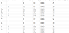
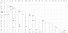
The J-M distances were computed to determine the class separability for the Landsat-8 OLIoptical images alone (Table 6) or combined with RADARSAT-2 SAR images (Table 7).The Landsat-8 images produced high separabilities, with a mean J-M distance of 1.968.There were 16 class pairs that showed a J-M distance of less than 1.85, indicating there is slightly higher separabilities than in the Wager Bay North study, which had 21 class pairs showing a J-M distance of less than 1.85 [8]. The minimum J-M distance was 1.101 and occurred between marine sand (Ms) and alluvial terrace (At). This is consistent with the findings of the study done in the Wager Bay North region, for which the minimum J-M distance was between marine clay (Mc) and alluvial terrace (At) [8]. So both study areas show low J-M distances between a marine sediment and an alluvial terrace sediment, however there is a slight difference in the type of sediment (sand vs. clay).This difference is probably due to the fact that the training areas used in this study include slightly different types of surficial classes, as mentioned above. However, similar to Byatt et al. [8], the minimum J-M distance of 1.101is higher than the values of0.75 reported by Shelat et al. [7], and 0.50 reported by LaRocque et al. [3]. Each of these studies used Landsat-7 ETM+ optical images, which do not have the same spectral resolution as the Landsat-8OLI images. This study also includes images acquired under both wet and dry surface conditions, which have been shown in Byatt [24] to improve the class separability.
J-M distance: Minimum = 1.101; Mean = 1.968;Maximum = 2.
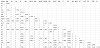
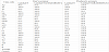
J-M distance: Minimum = 1.961; Mean = 1.999; Maximum = 2.
Once the RADARSAT-2 SAR images were combined to the Landsat-8 OLI images, the J-M distances increased dramatically. There were no class pairs having a J-M distance of less than 1.95 with most values above 1.99. The mean increased to 1.999 and the minimum to 1.961 between sand and gravel (SG) and thin marine sediment over bedrock (Ms/R). Even the Marine clay (Mc) class did not show any confusion with a value of 2.0 for all class comparisons. This indicates that the addition of RADARSAT-2 data improves substantially the separation between classes. This is consistent with the findings of the study in the Wager Bay North area, which showed a similar increase in J-M distance once the RADARSAT-2 data was added to the image combination [8].The minimum J-M distance (1.857) from the northern region was between Boulders (B) and Thin till over bedrock (T/R). This value was lower than the one computed in the south area (1.999) probably because of poorer training area selection, poorer image quality, or because the considered classes have a lower spectral separability.
5.2 Classification accuracies
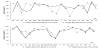
The overall classification accuracy (or out-of-bag accuracy) produced from the Landsat-8OLI data alone was 96.7% (Table 8).This is slightly higher than what was produced from the Wager Bay North study (92.8%) [8].These accuracies are much higher than the classification accuracies produced from comparative studies using Landsat optical data alone over similar northern terrain in Shelat et al. [7, 80.3%], Grunsky et al. [5, 84.8%], and LaRocque et al. [3, 86.2%]. It is also much higher than the accuracies produced by Campbell et al. [36, 46.3%] and Wityk et al. [37, 62.2%] for areas north of Wager Bay. This observed improvement in accuracy could be explained by the use of RF as a classifier, as opposed to the MLC classifier used by all previous studies. It could also be caused by the better spectral resolution of Landsat-8 OLI images compared to Landsat-5TM or Landsat-7 ETM+ images used in all previous studies. Incontrast to all the other previous studies, the classification included topographic (slope and DEM) data, which were consistently ranked as the strongest predictors in the RF variable importance plot (Figure 4a), such as in Byatt et al. [8]. This was also the case for the third most important variable, the near-infrared (NIR) band.

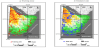
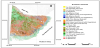
When the RADARSAT-2 data were added to the Landsat-8 data, the overall classification accuracy (or out-of-bag accuracy) improved to 99.3%.The resulting classified image is shown in Figure 5. The minimum accuracy is related to the Alluvial plains (Ap) class with 95.0% user’s accuracy (Table 9), which is much higher than the minimum value, when Landsat-8 images were used alone (90.0%). This class was confused with Marine clay with vegetation (McV) and Sand and gravel with vegetation (SGV), but the confusion was minimal. The improvements with adding SAR imagery were already observed in the previous studies, but the observed improvement was better than in Shelat et al. [7, 84.0%], Grunsky et al. [5, 91.9%] and LaRocque et al. [3, 90.8%] and in the Wager Bay North study of Byatt et al. [8, 98.1%]. This increase in accuracy is attributed to the high sensitivity of RADARSAT-2 to surface roughness and to the presence of moisture in the surficial materials. The rankings of importance from this image combination (Figure 4b) were similar to the rankings from the Landsat-8 image alone, with DEM and slope ranked as the most important data in the classification process followed by Landsat-8 Band 5 (near infrared - NIR). Each class has unique elevation slope conditions and the NIR reflection is particularly sensitive to variations in biomass which can directly point to different vegetation densities on the underlying surficial materials. Allof the RADARSAT-2 images were highly ranked, with 5 of the Landsat-8 bands being ranked last. Among all the RADARSAT-2 images, the RADARSAT-2 (A2 HV Wet) image was ranked the highest. The RADARSAT-2 HV image collected in wet conditions can capture difference in moisture conditions and is very sensitive to the vegetation covering the surficial material, which is important in separating various material classes. This indicates the importance of adding RADARSAT-2 data into the classification process for this particular study area.
5.3 Mapping accuracies
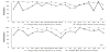
When only the Landsat-8 images are used, the overall mapping accuracy (Table 10) is lower (68.5%) than for the Wager Bay North region study (76.4%). This is also true for most class accuracies except for Af, MsV, sT, Tv, and B for the user’s accuracy (Figure 6a) and for Af, Mc, Ms, SGV, gsT, and TV for the producer’s accuracy (Figure 6b). When RADARSAT-2 images were added to the classification, there was a significant increase in the overall mapping accuracy (76.1%) and in the class user’s accuracy (Table 10). This is also true for the class producer’s accuracy of all the classes, but Ap, Af, Ms, gT, and T/R (Table 10). However, such as for the overall accuracy (93.3%, Byatt et al. [8]), both the user’s and producer’s accuracy for most of the classes remained systematically lower than in the Wager Bay north study (Figure 7).
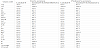
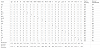
The classes with the low user’s accuracies are S/R (11.1%), T/R (53.3%), At (55.6%), R (60.6%), O (61.1%), Ap (63.6%), and gT (72.7%) (Table 10). The corresponding confusion matrix (Table 11) shows that S/R is mainly confused with SGV, T/R is mainly confused with R and SGV, At is mainly confused with Ms, R is mainly confused with Ms/R and SGV, O is mainly confused with McV and TV, and gT is mainly confused with O, SG and bT. For the producer’s accuracies, the low accuracies occur for S/R (20.0%), SGV (47.4%), SG (51.4%), O (64.7%), gT (72.7%), T (73.1%), and Mc (73.3%) (Table 10). The confusion matrix of Table 11 shows that S/R is mainly confused with R and T/R, SGV is manly confused with R, while SG is mainly confused with Ms and R.
Adding RADARSAT-2 in the classification helps discriminating between several classes. For example, when using Landsat-8 alone, the lowest J-M distance (1.1) occurring between At and Ms increased to 1.99 with the addition of the RADARSAT-2 images (Tables 6 and 7). Indeed, At (Figure8b) and Ms (Figure 8c) have similar spectral signatures, but slightly different roughness characteristics, with Ms having a somewhat smoother surface than At, resulting in less radar backscatter. This is also the case between Ap (Figure 8a) and SG (Figure 8e), for which the J-M distance increased from 1.59 to 1.99, Both classes have similar spectral signatures, but SG has a smoother surface resulting in low backscatter. The J-M distance between Ms (Figure 8c) and Mc (Figure 8d) improved from 1.64 for just Landsat-8 to 2.0 when the RADARSAT-2 images were included. Both classes present similar spectral response, but entirely different radar responses due to roughness and topographic variations which imparts a unique texture for this class on the SAR imagery. In addition, one can see the contribution from the slope image for separating Mc which drapes the glacial landscape and is characterized by various slopes and directions imparting a unique slope signature for this class.
The J-M distances between T/R (Figure 8i) and SGV (Figure 8f) increases from 1.67 to 1.96 when RADARSAT-2 are included in the classification. The distinct difference between roughness and vegetation/moisture characteristics can be seen when comparing both figures. The rough surface of T/R (Figure 8i) results in high backscatter on the SAR image, whereas SGV (Figure 8f) presents a smoother surface with far less backscatter. The same can be said when separating T/R from R, as the J-M distance improves from 1.42 to 1.96 when RADARSAT-2 are included in the classification. Bedrock outcrops (Figure 8j) present a much smoother surface to the radar than T/R (Figure 8i), resulting in less backscatter. The J-M distance between bT and T improved from 1.47 to 2 when RADARSAT-2 images were included in the classification. bT (Figure 8h) presents a much rougher surface resulting in slightly higher backscatter than T (Figure 8g).
These mapping accuracies obtained by comparing the classified image to ground observations (Table 10) are lower than the classification accuracies obtained by comparing the classified image to training areas (Table 8). This is expected due to the differences in scale between the imagery and the geologists’ observations on the ground as well as how the training areas characterize the terrain using only topography, vegetation and moisture, roughness and spectral variations compared to how the geologist synthesizes the scene from ground level with respect to the classes of interest. Because of the same scale difference, our map can have some localized differences with the surficial geology map established from field observations and the surficial geologist knowledge of the area [23]. For example, the coarser grained till classes (bT, gT, and gsT) should occur closer to the ice divide. Marine sand classes are sporadically misclassified south of Wager Bay in NTS 56H and 46E since they occur above the marine limit that was delineated from field observations (see Randour et al. [19], such as in the lowlands surrounding Roes Welcome Sound). As a result, large areas of bare bedrock along the coast of Roes Welcome Sound are mapped as sand and gravel or as thin marine sands over bedrock. Whilesome of these discrepancies may explain the lower mapping accuracy in the southern region compared with the Wager Bay North study, these accuracies are comparable, and indicate that the methods are applicable to other similar regions in the Arctic.
6. Conclusions
A surficial materials map was produced with 22 classes for an area located south of Wager Bay, Nunavut using Random Forests, a non-parametric classifier, applied to a combination of RADARSAT-2 C-band dual- polarized (HH and HV) and Landsat-8 OLI images with a digital elevation model and slope data. The addition of RADARSAT-2 C-HH and C-HV images to the classification greatly increased the overall classification accuracies to 99.3% compared to 96.7%, from using only Landsat-8, DEM, and slope data. For all the classes (but few), the user’s and producer’s class accuracy increased when the RADARSAT-2 images were added to the classification, leading to a class accuracy higher than 95% in most of the cases. This increase in accuracy shows the importance of including the RADARSAT-2 into the classification.
The resulting maps were compared to 648 georeferenced sites with field observations or interpreted from aerial photographs/Google Earth to determine the mapping accuracy. It increased from 68.5% when Landsat8 images were used alone to 76.1% when RADARSAT-2 images were added. Mapping accuracy was lower in the Wager Bay South study than in the North study possibly because of a lower number of georeferenced sites for comparison, specifically ground stations. The general increase in accuracies however, both classification and mapping, indicate the importance of addingRADARSAT-2 data. The type of RADARSAT-2 data used in this study is limited to images with an incidence angle between 20° and 49.3°, and only C-HH and C-HV bands. The work of Shelat et al. [7] showed the importance of including a variety of incidence angles (shallow, medium, and steep) in surficial material mapping, as it can increase class separability and classification accuracies. The inclusion of adding VH and VV images could also increase the classification accuracy, as it would add in more data for the classification process to work with. There is also the possibility of including polarimetric data, which can be derived from RADARSAT-2, to examine the potential of this new data source in mapping surficial materials.
Competing Interests
The authors declare that they have no competing interests.
Acknowledgments
The author is thankful to Deborah Lemkow (GSC) for helping with RADARSAT-2 image ordering: Roger Paulen for his careful review of the manuscript. Thanks to the anonymous reviewers.