


1. Introduction
The use of underground space for engineering systems has been increasing worldwide. Structural design of underground works is a process that takes into account various aspects which depend on the specific nature of the works. It covers the conception stage - choice of the site, location and orientation, and shape and geometry of eventual cavities; and the calculation stage - determination of structural solutions for achieving a certain performance. A great effort is made to ensure safety of the works, and each step is taken to integrate advances in various fields, like site investigation, hydromechanical characterization, computer modelling techniques, monitoring techniques, theory of structural safety and other theories [1,2].
Underground geoengineering is characterized by complex, uncertain geology and geomechanics that present challenges and require new tecniques to be dealt with. Problems are mainly related to heavy overburden which causes high levels of stresses and temperatures leading to a difficult geological environment that requires complex engineering design [3-6]. Special cases of the use of the deep underground are related to petroleum engineering, nuclear waste disposal, storage of products and energy, storage of CO2, geothermal energy, and these pose specific problems due to the environmental consequences they may have in case of failure.
The majority of underground construction projects have been completed safely. There is, however, an intrinsic risk associated with underground construction, since much is largely unknown. For example, several accidents have occured in various tunneling and mining projects that have resulted in delays, cost overruns, and in a few cases more significant human consequences such as injury and loss of life. As is common with problems in construction projects, these have been widely publicized, and pressure has been mounting from society to eradicate these accidents. There is, therefore, an increasing urgency to assess and manage the risks associated underground construction [7-10]. Most accidents in underground construction are associated with uncertainties. It is therefore essential to develop risk analysis systems.
Historically, risk assessment and risk analysis have not assumed particular relevance when evaluating underground projects and other major geotechnical projects. This has been changing, and risk analysis has been recently successfully implemented in major transportation infrastructures projects in UE, USA and Switzerland, using both commercial and research software for risk analysis. Special reference can be made to the Decision Aids for Tunneling (DAT), developed at the Massachusetts Institute of Technology in co-operation with Ecole Polytechnique Fédérale de Lausanne [11]. DAT is an interactive program that uses probabilistic modeling to analyze the effect of geotechnical uncertainties and construction uncertainties on construction costs and time through probabilistic modeling. Recent developments were introduced allowing dealing with other structures like embankments, bridges and engineered geothermal systems.
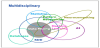
Prediction of geotechnical formation behavior in geoengineering is complex because of the uncertainties associated with the characterization of rock masses. In large projects, there is often a great amount of geotechnical data available which can help in reducing uncertainties in, for example, design values for the parameters [12]. The data can hold valuable information such as trends and patterns that can be used to improve decision making and optimization processes. It is however necessary to define standard ways of collecting, organizing and representing the data. Artifical Intelligence (AI) tools and pattern recognition techniques enable one to analyze datasets to retrieve information there. These are Data Miniming (DM) techniques [3,13-16]. DM is an area of computer science that lies at the intersection of statistics, machine learning, data management and databases, pattern recognition and artificial intelligence. The formal and complete analysis process is called Knowledge Discovery from Databases (KDD) that defines the main procedures for transforming data into knowledge [17-18].
This paper focus on the use of DM techniques in underground design and construction. After discussing the general challenges associated with deep underground engineering, and the application of AI and DM techniques in underground construction, the paper presents case studies where innovative DM-based techniques were developed and applied by the authors to address issues associated with deep undergound construction. In particular, the paper demonstrates the application of DM to the design and construction of a large and deep underground hydroelectric scheme, an underground laboratory, and undergound mining.
2. Challenges of Deep Underground Engineering
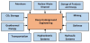
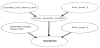
The use of deep underground space for engineering systems has been increasing due to urbanization. This is true for transportation systems, namely in road and railway transportation; in energy systems related to renewable energy, like hydropower and geothermal energy, as well as energy storage. It is also true for disposal of nuclear waste, storage of CO2 as well as of liquid and gaseous hydrocarbons, to water supply systems, for deep underground research laboratories, and of course for underground mining [1-2,4-6,19-21]. As such, there is a need for more rigorous rock engineering studies in the framework of different types of projects of deep underground engineering, as indicated in Figure 1.
In this section we provide illustrative examples of important underground projects worldwide and the associated challenges.
2.1 General projects
Nowadays, transport systems play an important role in supporting the integration of several regions and countries like in EU. Tunnels are very important within transport infrastructures. In railway tunnels, the construction of very long and deep railway tunnels was already performed with Gothard base tunnel in Switzerland (57.1 km), Seikan tunnel in Japan (53.9 km), Channel tunnel in UK and France (50.5 km), Yulhyeon in South Korea (50.3 km) and Songshan lake tunnel in China (35.4 km). Are now under construction extensive tunnels, like Brenner base tunnel in Austria (55 km) and Lyon-Turim base tunnel in France and Italy (52 km) [9,22-23]. In road tunnels, reference is made to the Laerdal tunnel, in Norway, the longest one with 24.5 km in extension, to the Yamate tunnel in Japan with 18.2 km and to the Zhongnshan tunnel in China with 18.02 km. Very long water tunnels were already constructed like Delaware Aqueduct in USA with 137.0 km and the Paijanme tunnel in Finland with 120.0 km. Several severe accidents occurred in some of the mentioned tunnels. As examples, large quantities of underground water causes flooding in Seikan tunnel; and collapses occurred at Fadio zone, Gotthard base tunnel, caused by squeezing ground that let to excessive deformation and led latter to partial collapse of the lining [9,24].
In deep mining activities the major problems are associated with large deformations and rockburst due to overstressing of the rock mass caused by excavations at great depth. Comprehensive investigations of deep mining mechanics are of great interest. In coal mines, several types of events were identified and classified [25]. The accidents can cause loss of live, equipment damage and damage to the tunnel structure that may lead to a collapse. Nowadays, coal mines reach depths between 1,200 to 1,400 m in China and in some European countries, and more than 3,000 m for gold mines in Brazil and South Africa [26]. The coal resources play a leading role in the energy strategy in China, and represents about 70% of the total energy consumption. Deep coal resources below 1,000 m represents an important part [27]. At the beginning of the 21st century large deformation failure problems become more challenging with increasing of depth. This was basically considered because the traditional 121 method was not suitable for deep mining purpose. The theory of CCBT (Cutting Cantilever Beam Theory) was put forward and provided the basis for the non-pillar, under which the 110 mining method was developed [28].
Regarding CO2 storage activities, various technologies have been developed over recent years to address the increasingly urgent demand for the protection of the Earth’s atmosphere from ozone depleting emissions, and ensure sustainability. This is true for different gaseous emissions, most significantly for carbon dioxide (CO2), where significant advances have been made in the processes of emissions reduction. Furthermore, it is no longer acceptable to simply reduce (or eliminate) emissions, but rather capture and store atmospheric CO2 in processes that lead to an overall reduction of the atmospheric CO2 resulting in carbon negative facilities, cities and counties. Different options for carbon capture, utilization and storage (CCUS) technologies exist and have been or are in the process of being implemented worldwide [3,29-30], take into account not only energy demand but also environmental requirements. In general, it is now accepted that CCUS is a viable technological solution to reduce GGH emissions and can be introduced as a strategy within the larger context of climate change policies [29-31].
With these technological advancements, the economics of large, commercial scale CCUS schemes has become more viable. This is particularly true when governmental entities use policies in place that promote CCUS such as carbon credit incentives (as opposed to but possibly coupled with taxation on carbon emissions). More recently, much research is being conducted on innovative techniques to increase the financial viability of CCUS such as the use of the captured carbon in enhancing the recovery of oil and gas fields where conditions are favorable. Continued research in every stage of the CCUS process is only likely to decrease costs and make CCUS more economically viable.
Despite these advancements, CCUS, as with any operation in the underground is uncertain. These uncertainties come from various sources, and there are hazards and risks associated with them. The storage of CO2 in deep onshore and offshore geological formations uses many of the technologies developed by oil and gas industry, and can be coupled with enhanced oil and gas recovery schemes (EOR and EGR) and in saline aquifers (Figure 2), [29-36]. CO2 can also be stored in coal beds, particularly in unminable deep coal seams and well-sealed abandoned coal mines [36]. CO2 should be safely injected and stored at well characterized and properly managed sites to ensure the long-term safety of a geologic CO2 storage project [30,37-38]. CO2 is injected in deep geological formations where conditions of pressure and temperatures are favorable for CO2 to exist in the so-called supercritical or liquid form, requiring less volume than in its gaseous form [29]. Adequate planning of the injection and storage processes is essential to ensure safety with no CO2 leakage during the entire storage period. At depths below about 800-1,000 m, CO2 has a liquidlike density, which makes the potential use of porous sedimentary rocks as underground reservoirs possible.

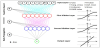
There are different possibilities for geological sequestration as illustrated in Figure 3 [35-39]. Several geological solutions (closed systems) can be considered as feasible, such as depleted oils and gas reservoirs, deep saline aquifers, shale gas, coal seams, abandoned coal mines, among others. Coal seams and abandoned coal mines are currently being used to produce enhanced coal bed methane (ECBM), as well shale as gas technologies which can be viable in terms of permanent CO2 disposal [30,39-40].
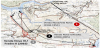
2.2 The Jinping II hydroelectric scheme, China
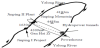
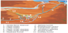
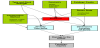
The first example is the Jinping II hydroelectric project constructed recently in China. Jinping II is a project by Ertan Hydropower Development Co. Ltd and is located in Yalong River. Jinping site is unique in that it utilizes a natural 180-degree bend in the Yalong River (Figure 4). Jinping II has a large underground complex for the powerhouse with 8 units and a total installed capacity of 4,800 MW, to produce a multi-year average annual output of 24.23 TWh. The construction started in August 2008 and the powerhouse was finished in 2012. The project, includes four high pressure tunnels 16.67 km long, with a 60 m spacing between them, a drainage tunnel, two access tunnels, and a large underground powerhouse structure [4,10,41]. Two of the high pressure tunnels are excavated using drilling and blasting (D&B), and the other two excavated using tunnel boring machines (TBM). The construction of the tunnels for the high pressure circuit and associated auxiliary tunnels and drainage tunnel was the most challenging portion of the project. Figure 5 summarizes some of the issues faced during the construction of the high pressure hydraulic circuit of Jinping II [10]. These consisted mainly of rockbursts, waterbursts and large deformations.
The depth of the overlying strata was between 1,500-2,000 m, with a maximum of 2,525 m. Rockbursts were observed in deep marbles due to the significant depths and large diameters of the extensive tunnels. A very severe rockburst occurred on November 2009 during the excavation of the drainage tunnel by using Robbins TBM. This rockburst was responsible for the destruction of the main beam of the TBM and an area of about 30 m behind the cutter head [4]. As a consequence the Chinese Society for Rock Mechanics and Engineering organized a Consulting Workshop in 2009 to review and discuss the geotechnical problems faced during the construction of the at Jinping II tunnels, with particular emphasis on the occurrence of rockbursts. Several reports were produced focusing on the rockburst problem [41-46]. These reports contained estimations of in situ stresses, the geometry of the excavations when using D&B method, modelling and especially rockburst prediction as well as suggestions on how to mitigate the TBM problems. Another important consequence was the creation of a database containing information regarding the rockburst events that occurred at Jinping II. The data was used, by applying DM techniques to develop models to predict the probability of occurrence of rockbursts and their characteristics: type, location, depth and width, and time delay [46].
During the excavation of Jinping II diversion tunnels 1 and 2 at depth between 1,550 and 1,860 m, a chlorite schist formation was encountered [4,47]. The stresses were about 41-50 MPa (Figure 5). The geological conditions were complex and the lithology frequently changed. Large deformations occurred and two serious collapses happened due to the use of inadequate support systems. Laboratory tests were performed to characterize the physical and mechanical properties of the chlorite schist and an elastic-plastic constitutive model was developed. For stability control and support optimization, an improved support system was adopted to control large deformations and an over-excavation approach was followed [4,47].
Finally, because of the fracture and karst nature of the terrain, several waterbursts of high pressure groundwater occurred during the construction of the tunnels [9]. Karst related waterbursts were predominant at ends of the tunnels as illustrated before in Figure 5. Figure 6 shows an image of a waterburst during the excavation of one of the access tunnels. Ground water treatment was necessary to mitigate waterbursts [4].

2.3 The Venda Nova hydroelectric scheme, Portugal
In Portugal, investiments in renewable energies have significantly increased in the last decades, particularly in sun, wind, and hydropower from dams by pumped storage systems. Some of the new hydropower systems derived from the repowering of existing schemes. This technology permits storing energy during the periods of low demand. This is the case of Venda Nova hydroelectric scheme [48]. Two new schemes were built to complement the Venda Nova/Vila Nova power scheme built in the 50’s: Venda Nova II was completed in 2005 and Venda Nova III in 2016 as shown in Figure 7. Both schemes are underground connecting Venda Nova and Salamonde reservoirs with extensive hydraulic circuits and deep underground cavern complexes.
The scheme of Venda Nova II is almost fully comprised of underground facilities, including caverns and several tunnels and shafts (Figure 8) [49]. A large dataset was generated that consisted of the results of the application of the empirical systems and results from laboratory (uniaxial compressive strength and sliding of discontinuities) and in situ tests (Small Flat Jacks – SFJ, Large Flat Jacks – LFJ and dilatometers) [12,49]. The database was large enough to be mined. Prior to doing so, it was necessary to clean the data to remove duplicated records. The reduced number of some tests hindered the possibility to include them in data mining process because it is important that, for each type of input variable, a large amount of data exists. Data were organized and structured in a database composed by 1,230 examples and twenty-two attributes which were analyzed by applying DM techniques.
2.4 Underground laboratory at DUSEL, USA
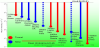
Underground laboratories are important deep underground structures that have to be considered. They can include existing infrastructures to host physics experiments [50-56]. Such laboratories include INO in India and of course DUSEL in the USA and CJPL in China [51,57-58]. A comparison of the main underground laboratories is indicated in Figure 9.
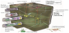
The National Science Foundation (NSF) in USA choose Homestake as the location for an underground laboratory. The project was known as DUSEL (Deep Underground Science and Engineering Laboratory) project. The laboratory was seen as a multi-discipline facility with particle physics providing the lead but other disciplines being a significant part of the facility, including geomicrobiology, geosciences, and geoengineering. The possibilities for how the nonphysics sciences would participate were described in detail in the EarthLab report to the NSF [19]. A representation of DUSEL is illustrated in Figure 10. Because some of the physics experiments being envisioned, the laboratory required large cavities at depth, for example, right circular cylinders with dimensions of as much as 86 m high and 60 m in diameter at a depth of about 1.5 km below the surface (4850 Level). A geotechnical investigation program was undertaken as part of the site characterization [51]. The Laboratory is located in the Precambrian core of the Black Hills of South Dakota. The geologic units exposed in the main campus at the 4850 Level consist of Precambrian metamorphic rocks that are intensely folded and plunging steeply to the southwest. From oldest to youngest, they include a metamorphosed basalt (now an amphibolite) known as the Yates Unit, the Poorman Fm., a metasedimentary units consisting of phyllites and schists, and rhyolites intruded during the Tertiary Period. Using a database of geomechanical information gathered in the scope of the DUSEL project, new geomechanical models for the prediction of rock mass quality indexes, namely RMR, Q and GSI were developed using DM techniques [59].
3. Artificial Intelligence Techniques
AI techniques are progressing very rapidly since 1956. AI today is labeled as a narrow when it is designed to perform a specific task or labeled general when designed to outperform humans at a very cognitive task [60]. In the area of deep underground engineering, tasks are for the most part narrow. The prediction of geotechnical formation behavior in geoengineering is complex because of the uncertainties in characterizing rock masses. In large projects, the great amount of geotechnical data that is generated and collected can be used to reduce uncertainties [12].
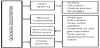
Data can hold valuable information such trends and patterns that can be used to improve decision making and optimize processes. Therefore, it is necessary to define standard ways of collecting, organizing and representing data. There are automatic tools from the field of AI and pattern recognition that enable one to analyze and interpret data using DM techniques [13,15-16]. DM is an area of computer science that lies at the intersection of statistics, machine learning, data management and databases, pattern recognition, artificial intelligence and other areas (Figure 11).
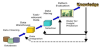
KDD is a formal and complete analysis process that defines the main procedures for transforming data into knowledge. The KDD process consists in the following steps [13,49,61] (see Figure 12): collection of target dataset; data warehousing; data are transformed in appropriate forms for the DM process; selection of DM tool; relationship identification of DM (classes, clusters, associations); interpretation of results; and consolidation of discovered knowledge. There are several DM techniques, each one with its own purposes and capabilities, namely KBS systems, Decision Trees and Rule Induction, Neural Networks, Fuzzy modeling, Support Vector Machines, K-Nearest Neighbors, Bayesian networks (BN), Learning Classifier Systems and Instance-Based Algorithms [49,62-64].
Studies using a formal KDD framework are still not common in rock mechanics related activities, however when applied they can provide important insights into the most influential parameters on the behavior of rock masses. A application of this is a study done for the DUSEL laboratory (Figure 10) [19], where innovative regression models, using different DM techniques, were developed to determine geomechanical indexes for the project [59]. One of the most important tasks in the KDD process is the DM step which consists of choosing a learning algorithm for training and ultimate build a model that represents the data. Once the training phase is completed, the obtained model will be evaluated using a test data set that has not been used during the learning process. The results consist of several different models however there is no universal one to efficiently solve all the problems.
A brief overview of the techniques used in our studies is presented next. A Decision Tree (DT) is a tree like graph that represents a set of rules for classifying data. These rules can be learned by using a classlabeled training data set [49,59]. Artificial Neural Networks (ANN) are deep learning techniques modelled after how neurons operate within the human brain [12]. They are formed by groups artificial neurons connected in layers, where signals travel from the first (input) to the last (output) layer, similar structure to the brain neurons. These networks, which can be learned from data, are particularly useful in complex applications, to recognize patterns and to predict future events. The technique of Support Vector Machine (SVM) are supervised learning models normally used for data classification and regression analysis. Given categorized training data, SVM determine an optimal plane that defines the decision boundaries, i.e. the distance between classes [65]. Finally, Bayesian networks (BN) are graphical representations of the joint probability of a certain domain under certain simplifying assumptions [9,66].
The increasing interest in DM causes the need to define standard procedures to carry out the analysis. In this context, the two most used methodologies in DM are the CRISP-DM (Cross-Industry Standard Process for Data Mining) and the SEMMA (Sample, Explore, Modify, Model, and Assess). The CRISP-DM methodology was developed by a group of companies. It is an iterative and interactive hierarchic model which develops in several phases [67], (Figure 13). The SEMMA methodology was developed by the SAS Enterprise Miner institute which delivers services in the areas of DM and decision support [17,49].
Several works have already applied DM techniques in deep underground space.
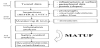
One such work relates to tunnel management and maintenance for old tunnels [62]. A KBS system named MATUF was developed and techniques for modelling decisions under uncertainty based on BNs were used. Figure 14 indicates the levels of information in the system MATUF and Figure 15 illustrates a BN for water presence problems.
Abdulla et al. [68], proposed an innovative ANN based probabilistic classifier to obtain the probability gypsum presence in the subsurface with an application to Masdar City in UAE. ANN proved to be an efficient tool for spatial interpolation due to its noise immunity and complicated pattern recognition capabilities for the application of a metro line at Masdar city. Figure 16 illustrates the neural network used in the study.
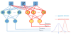
Another work that is related to coal mines is that conducted by Mahdevar et al. [69] for stability prediction of gate roadways in longwall mining using ANNs. Datasets of roof displacements monitored of a 1.2 km roadway in Tabas coal mine in Iran were setup in order to develop an ANN model. After several tests based on trial and error, a four-layer network with an input layer, two transfer functions in the first and the second hidden layers, and a linear transfer function in the output layer was found to be optimum. As indicated in Figure 17, seven and six neurons were introduced to the first and second hidden layers, respectively.
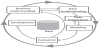
Another work related to coal mines is the study by Slezak et al. [70] on a decision support system for monitoring coal mine processes and predictive analytics of sensor readings. Hazard models were constructed, as well as functionalities responsible for data acquisition and storage, data cleaning and transformation. The architecture of the decision support system is presented on Figure 18. It consists of the following major components: Data warehouse; data preparation and cleaning module; and modules that utilize the data coming both from the data warehouse and directly from coal mine systems, mainly analytical, prediction and expert systems modules. The concept of methane concentration was divided into four fuzzy sets. Depending on the kind of sensor and its location, its status can be related to different values of methane concentration (Figure 19).
4. Underground Hydroelectric Schemes
4.1 Introduction to Venda Nova II
For deep underground hydroelectric schemes, analytical models can be developed using different sets of parameters for the prediction of variables of interest so that they could adapt to the level of knowledge concerning the rock mass and to the project development stage. The case of Venda Nova II presented before was chosen (Figure 7 and Figure 8). The goal was to develop models to calculate strength (friction angle - φ’; cohesion - c') and deformability of the rock mass (E).
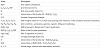
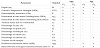
Geotechnical data were organised and structured in a database composed by 1,230 examples and twenty-two attributes which are described in Table 1. The attributes were mainly parameters of the empirical classification systems RMR and Q, the RMR class and the UCS of the intact rock [73-75]. From the original attributes, others were calculated including the geomechanical parameters by means of analytical solutions. The calculated geomechanical parameters were added to the database with other attributes to check their possible influence on the models. Globally, eleven new attributes were added. From this point, the geomechanical parameters obtained using this methodology will be called “computed values” while the ones obtained with the DM models will be called “predicted values”. It is important to mention that the “computed values” for the deformability modulus were calibrated with the results of reliable and large scale in situ tests, namely LFJ tests.
In spite of the high number of records within the database, there were some limitations. Considering the histograms of each variable of interest, the main limitations were: UCS>100 MPa, RQD values over 65 and slightly wet to dry rock mass. Therefore, the models developed in this work should only be applied to rock masses with similar characteristics.
The SAS software was used as the modelling tool [17]. The evaluation of the models was performed using the results provided by this software and complementary calculations on spreadsheets. In regression problems, the goal is to estimate the model which minimizes an error measurement between real and predicted values considering N examples. The error measures used were the following: MAD (Mean Absolute Deviation) and RMSE (Root Mean Squared Error) [49]. To validate and assess the models accuracy, the holdout method was used [12].
4.2 Calculation of deformability modulus at Venda Nova II
The deformability modulus (E) is an important input parameter in any rock mass behaviour analysis. For a more representative value of E, considering all factors, large scale in situ tests are needed. LFJ tests were performed and analysed [49,74]. However, most procedures found in the literature to estimate this parameter for isotropic rock masses are based on simple expressions related to empirical systems or other index values. Several empirical expressions were used for the calculation of E of the rock mass using DM techniques [12,49]. The expressions used in the study are given in the references [71-79].
To obtain one final value of E from the application of these expressions, a statistical methodology was established. For each case, the results of all expressions were computed, as well as their mean and standard deviation. The values outside the range of one standard deviation from the mean were eliminated and the mean of the remaining values was computed and considered as the final value of E. The values of E obtained by the described methodology were compared with the results of LFJ tests [49]. Table 2 presents some statistical results of this evaluation. The mean values obtained by both methodologies is similar (around 4% of variability). The main difference is the higher dispersion in the calculated values translated by a higher standard deviation which is normal because the LFJ tests are much more accurate in determining E than the empirical expressions. Thus, despite the higher variability, the calculated values match well to those obtained by reliable in situ tests and can be considered realistic predictions.

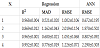
Preliminary calculations show that a logarithmic transformation ln(E) would improve the accuracy of the models. The main reason of this transformation was to avoid the prediction of negative values for E in poorer rock mass conditions, which was observed in some cases with the linear model. The parameters that produced the most accurate model were directly related to geomechanical indexes, namely the RMR and Q values. Additionally, these indexes assemble important information for the rock mass deformability prediction. These models can be used for the prediction of E when a thorough characterization of the rock mass is available. The results are the following: i) regression – R2=0.978±0.001; MAD=0.088±0.004; RMSE=0.137±0.009; ii) ANN – RMSE=0.141±0.016.
The regression model obtained is:
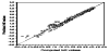
The linear regression model is very accurate, and even slightly outperforms the ANN model in terms of RMSE. Because ln (E) ranged from approximately -0.57 to 4.22, the error can be considered negligible for engineering practice. The model is stable for all ranges of observed values as shown in Figure 20. In terms of geomechanical coefficients, the RMR was the most important parameter for the calculation of E. Indeed, several regression models were tested but the most reliable models were based in this index. A simple correlation between E and RMR using all available data led to very acceptable results. The expression for this correlation was:
When only parameters related to the joints are available (P3, P3 and P3), which are also important parameters in the prediction of E, the procedure that leads to better results is first to calculate the RMR with a model based on these parameters [49] and second, using equation 1, to calculate the final value of E. Table 3 presents the results for these two methods. In both cases, there are no confidence intervals because the results were based on a simple correlation procedure using all data.
The correlation has the advantage of avoiding the Q index evaluation. However, it does not have the statistical validation present in the previous, more complex model. For the last method, the decreasing accuracy is much more significant, especially for E values corresponding to poorer rock masses (ln(E)<1 or RMR<34).
4.3 Developed models for strength parameters
Strength parameters were not originally present in the database, but were indirectly derived from available information using established analytical methodologies. Concerning the strength parameters, the main goal was to develop models to predict the Mohr-Coulomb parameters using different types of data. To obtain the values of these parameters to include in the database, the Hoek and Brown (H-B) strength parameters were firstly computed. Then c' and φ’ were derived by fitting an average linear relationship to the generated failure envelope formulated in terms of effective stresses [73].
The prediction models for φ’ and c' were developed considering a reference depth (H) of 350 m (the average depth of the main caverns of the powerhouse complex) and a disturbance factor (D) of zero. To allow for a simple and direct transformation of the values predicted by the models for other conditions (different H and D), a parametric study was performed. Based on this study, a generic methodology for transforming the geomechanical parameters for a given H and D to a different pair of values was developed and then particularised for the DM models. The generic methodology is based on the application of two correction factors, one for each parameter, and is described in Miranda [49].
Figure 21 shows a plot of the most important parameters in the prediction of φ’. There is a large number of variables related to the prediction of this geomechanical parameter with several ones showing similar importance. However, the most important variables are: (i) UCS, which was expected because this value is also a strength measure, and (ii) the Q index (with logarithmic transformation) and other variables related to the Q system. This is unexpected because the Q system is normally used only for classification purposes and not for the calculation of strength parameters considering the rock mass as a continuum medium even though the Jr/Ja ratio is already considered a strength index for joints. Nevertheless, the Q index is very complete and can be used for the prediction of geomechanical parameters [71].
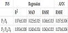
In this context, several sets of parameters were tested to obtain the best prediction models that could simplify the way φ’ is calculated. The input variable sets (IVS) which presented the best results were: i) IVS 1: all variables; ii) IVS 2: Q; log Q; Q’; log Q’; RMR; iii) IVS 3: all RMR parameters (P1, P2,…, P6); and iv) IVS 4: RMR parameters P1, P4 and P6.
Results for the different IVS are presented in Table 4. The expression for the regression model of IVS 4 is the following:
As expected, the models using IVS 1 were the most accurate. Nevertheless, the remaining models also had very good predictive performances. IVS 3, which uses all the RMR parameters, is only slightly outperformed by IVS 1. The error measures and R2 are very close. For a wide range of values, approximately from 35 to 63º, the prediction capacity is very uniform and reliable because the plotted values lie near the 45º line, even though a small accuracy reduction can be observed for the lower values of φ'. This range of values covers a great variety of possible weathering states of the granite rock mass from fresh rock to transition from rock to soil. IVS 2 presented the worst performance. In spite of using information from the RMR and Q coefficients, it was outperformed by the simpler models. For the case of φ', the use of specific information about rock mass characteristics presented better results than using overall quality indexes like the RMR and Q.
The most important RMR parameter was by far the one related to UCS, meaning that in granite rock masses, φ’ is closely related to this strength measure [12]. The variables related to joint conditions and orientation (P4 and P6, respectively) also appear to be good predictors. Even though a high importance of joint conditions was expected, the considerable weight of the parameter related to the joint orientation is not as acceptable. It can be due to limitations of the database or even of the RMR system itself which can overrate the importance of this parameter. Finally, IVS 4 uses these three parameters for the prediction of φ’ with very good results. Comparing with IVS 1 and 3, error measures are higher but the model has the advantage of being very simple because it uses only three parameters. Considering the MAD and RMSE values from Table 4, the mean expected error for these models is only about 1°, which can be considered negligible for engineering purposes.
The ANN outperformed the regression models for IVS 1 to 3 in terms of the RMSE and this is especially true for IVS 1, where the error was reduced by more than 30%. For IVS4, the RMSE of the ANN is 87% higher than the RMSE for the regression model. The ANN performs worst when using fewer parameters. Nevertheless, the RMSE of all the trained ANN were acceptable for every considered model, which means that they are highly accurate in the prediction of φ’.
tan (φ’) was also considered a target variable because of its physical meaning. The preliminary runs pointed to the significant importance of the GSI, which is normal because φ’ is indirectly dependent on this parameter. Moreover, the RMR parameters, mainly the one related to UCS (P1) and some parameters related to discontinuities (P4 and P6) were significantly important. Table 5 present the overall performance of both models.
The results are very similar to those obtained for φ’ with the same sets of parameters. When using all RMR parameters, the value of φ’ can be estimated with acceptable accuracy even though there is a slight loss of accuracy for lower values compared to the remaining range. As expected, the consideration of only the three most important parameters increases the mean errors, but the models have the advantage of being simpler. In both cases, and considering only the RMSE, the multiple regression models outperformed the ANN in the prediction of the target variable. Also a correlation between tan(φ’) and E was found:
The correlation presents the intrinsic interest of allowing the evaluation of a strength parameter from an estimation of a deformability parameter and vice-versa.
Finally, models for cohesion (c’) prediction were developed and the obtained results are detailed in the publications [12,49].
5. Underground Laboratory
DM studies were performed for DUSEL, located in South Dakota, USA [59,80], (Figure 10). Detailed geological and geomechanical studies were performed at 4850 Level (about 1,470 m deep) and at 7400 Level (about 2,240 m deep) [51,53,81].
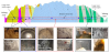
A mapping program for the 4850 Level was conducted by LFA [81], and this focused on a triangle of drifts and included a total of 1,300 m of detailed mapping (Figure 22). Site mapping focused on the detailed evaluation of the existing excavations, geological structure (discontinuities, foliation planes, shear zones, inflows, etc.), hydrogeology (water seepage), and rock alteration. Initially, approximately 1,820 m of drifts were proposed to be mapped. At the initiation of the mapping, it was decided that increased detail was needed and, therefore, the focus shifted to the primary area of interest, which is the triangle of drifts between the Ross and Yates Shafts up to the Yates and Poorman contact in both drifts. Based on the manually collected data, a geotechnical evaluation was conducted to delineate the dominant discontinuity sets within the drifts and to further characterize the rock mass. The data collected were also used in calculation of RMR and Q values along the drifts that were mapped. GSI values were estimated regularly based on structure and surface conditions of the rock mass. Initially the rock mass was subdivided on 11 structural domains. However, taking into consideration all the information included in the report of LFA, the database gathered is mainly composed by the weights of the RMR and Q empirical systems application and the GSI values in a total of 127 cases gathered in the different domains. Figure 23 shows attributes used in the database.
This work was related to the development of new models based on DM techniques to predict the values of RMR, Q and GSI with less information than the original formulations in which the evaluation of several parameters was necessary. These models can be helpful in geomechanical characterization conditions where information is scarce, uncertain or difficult and expensive to obtain. In this sense, these models were especially well suited in the preliminary stages of design.
For each index, the study starts with the computation of the parameters with main influence in their prediction. Then, the models are developed using only the minimum amount of input parameters that lead to acceptable results from an engineering perspective. The DM algorithms used in this study were the MR, ANN, and SVM. Only the MR provides an equation relating the output and the input variables. The MR is similar to the simple regression with the main difference being the number of independent variables involved. The simple regression involves only one independent variable whereas the MR involves several independent variables and establishes a relationship among them and the dependent variable. The ANN uses a human brain like structure composed of simple processing units, denominated nodes or artificial neurons, with a large number of interconnections. The multilayer perceptron architecture was adopted in this work [82]. The SVM was originally used in classification problems [83]. The basic idea was to separate two classes of objects using a set of functions. This process is called mapping and the functions are known as kernels. The planes that separate the classes are known as hyperplanes and there is an optimization iterative algorithm to find the hyperplane which establishes the largest separation between classes. The vectors placed at the nearest distance in both sides of the hyperplane are denoted support vectors. Both in classification and regression methods there is an error function to minimize subjected to some constraints.
The modeling software used was the R program [84] together with the RMiner [85] package that allows one to apply the DM algorithms and to evaluate their performance under a different set of metrics. In this work the metrics MAD and RMSE were used. To evaluate the algorithm performance, a cross-validation [86] was applied. In this method the examples are divided into 5 subsets with approximately equal number of records. Ten runs are performed using 4/5 of the records for training and 1/5 for testing rotating the subsets using for training and testing. The final metrics are the mean of the metrics obtained in the 10 runs.
The relative importance of each input parameter was also evaluated by applying a sensitivity analysis [87]. This is carried out after the training phase and is intended to evaluate the response of the model when the input parameters are changed. The importance of a given input parameter is evaluated by changing its value from a minimum to a maximum and at same time maintaining the remaining input parameters at their mean values.
It was concluded that the most important parameters in the prediction of RMR were the weights related with the RQD, joint spacing and underground water for every DM algorithm (P2, P3 and P5) [59]. Very accurate models were obtained using only these three parameters and even with only the two most important ones (P2 and P3). For the GSI index it was observed that the models should consider at least the three most important input parameters. Similarly to RMR, it was possible to use models for the prediction of the Q index using only two or three parameters and maintaining a high predictive accuracy [59]. The metrics for the RMR and Q indexes with two and three parameters are presented in Table 6. With exception of GSI, in every model a good distribution of the values around the 45° slope line between predicted and real values could be observed.
The application of DM intelligent methods consists of search and inference of patterns or models. BNs are another possibility that allows one to introduce uncertainties related to the geotechnical and construction aspects, risk management and decision making during construction. Several BNs were learned and tested on the database, using the software GeNIe. In this specific study, only models that allow predicting RMR values were developed. They were trained with about 4/5 of the cases and tested on 25 different cases. The algorithm used for learning the models was the “greedy thick thinning” with a uniform prior [88].
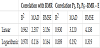
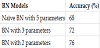
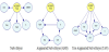
Figure 24 shows the structure of learned BN models obtained using five parameters (P1, P2, P3, P4 and P5), three parameters (P2, P3 and P5) and two parameters (P2 and P3). The learned networks were tested on cases from the database and results are shown on Table 7. Table 7 shows that when training and testing the models (the model fit), the best results were reached with the BN with 2 parameters where only P2 and P3 are used. This model assumes that, not only P2 and P3 are important in predicting RMR but that also the interrelationship between P2 and P3 (represented by the arrow) is an important element of the prediction.
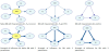
In the user interface GeNIe, it is also possible to calculate the strength of influence per arc, and represent this visually in the network. The strength of influence is determined by looking at the posterior probability distribution of a node, for each possible state of the parent or child node, depending on the type of connection, and calculation the distance all the differences between the conditional probability of a node given the parent node, and the a-priori probability of the node [89]. The strengths for the BN models are also shown in Figure 24. These strengths were calculated using the Hellinger distance [59]. Figure 24 shows that many of the correlations between the different variables show thick arcs, indicating they are strongly determined by the value of their parent nodes, i.e. a strong influence between variables. The strongest influences are between RMR and P3, RMR and P2 and P2 and P3.
6. Occurrence of Rockbursts
6.1 Rockburst events – laboratory experiments
There are several effective design methods available to deal with ground fall in mining. However, this is not the case for rockbursting and seismicity-related mine design problems. Modeling analyses are a fundamental tool to assess potential undesirable events and its cost is only a small fraction of the potential consequences to excavation operations. A large variety of numerical analysis methods can and have been applied to underground engineering in order to assess the potential for the occurrence of rockburst. Monitoring of seismic events and visualization techniques in deep tunnels and mining activities are very useful tools for predicting potentially hazardous situations in order to assist the construction in time. Rockburst is a type of event that can range from minor to significant volumes of rock falling or being ejected with high energy, which can have devastating consequences. These phenomena are commonly reported in deep underground mining structures, but can also occur in deep tunnels, such as the Jinping II hydroelectric scheme (Figure 5). A rockburst triaxial experimental system is important in predicting these types of events both in mining and in other deep underground projects, and previous analysis of rockburst test results have allowed the authors to develop predictive models to estimate rockburst maximum stress and a risk index [90-92].
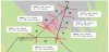
Rockburst is affected by different factors [9,92]. Figure 25 shows the influence diagram listing the factors that affected the probability of a rockburst as well as its potential consequences. These influence diagrams are very important in the design of DM models.
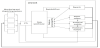
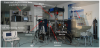
DM techniques were applied successfully to a rockburst laboratory test database obtained from tests at SKL-GDUE, China [90]. The developed triaxial rock test machine for modelling the rockburst is presented in Figure 26 [90-91]. The equipment is a true triaxial testing scheme. During the test, one surface of the specimen can be unloaded immediately from the true triaxial compression condition, simulating the stress condition of the rock mass at the free excavation boundary in underground excavations. It is a system for rockburst testing that includes the main machine, hydraulic pressure controlling unit and data acquisition for forces, displacements, acoustic emission (AE) and high speed digital recording. Normally, in the tests acoustic polarity transducers are used with a resonance frequency of about 150 kHz and a fairly flat response from 100-300 kHz [26,91]. The stress paths used by the testing system simulate the different types of rockburst that can occur. The AE characteristics are very important and can be used and analysed in order to understand crack propagation phenomena.
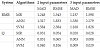
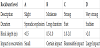
A database of 139 cases with samples from different rock types and from China, Italy, Canada and Iran was compiled. Two indices were developed and used, the rockburst maximum stress (σRB) and rockburst risk index (IRB). The meaning of these indices are described in detail in He et al. [91]. DM techniques were applied to the rockburst database to infer prediction models of the indices σRB and IRB. New models were established using the algorithms MR, ANN and SVM. Table 8 shows information for each field. The samples had a prismatic shape with an average length of 59 mm, with a minimum of 39 mm and a maximum of 111 mm. The volume had 312 cm3 in average.

All the tests were of the strainburst type. The rockburst critical depth He was calculated assuming a simplified circular shape in the crown of the tunnel, a concentration factor for the stresses equal to 2 and a specific weight of 27 kN/m3 for the overburden rock mass by the expression:
where σRB is the rockburst maximum stress obtained in the tests.
A rockburst risk index IRB was also calculated following the formula:
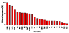
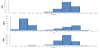
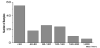
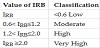
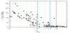
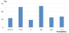
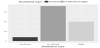
The rupture stresses σRB obtained in the tests have an average value for all samples of 82.6 MPa, with a minimum of 16.5 MPa for mudstone and a maximum of 161.4 MPa for granite. The average value of coal was equal to 19.0 MPa and for sandstone 101.4 MPa. Figure 27 shows the distribution of the rockburst stresses obtained in all samples. A large number of samples for soft rocks with values lower than 40 MPa were observed. The distribution for the classes for all tests and for the most representative rock formations (coal, granite and sandstone) are shown in Table 9 for the index IRB. Low IRB values were obtained in 56% of the samples, and very high values were 13% of the total. Figure 28 represents the relation between IRB and σRB. A logarithmic relation between IRB and K (ratio between average horizontal stresses and vertical stress due to overburden) was obtained [91].
In Table 10 four data groups were considered as input parameters for modeling and evaluation of both indexes. The DM algorithms used were also MR, ANN and SVM.
The results of σRB for group G1, with the principal variables, show good performances for all the developed models with error measures fluctuating approximately between 20 and 32 MPa for a variable that ranges from 10.6 MPa to 255.5 MPa (with a mean value of 82.6 MPa). Also the values of the correlation coefficient are rather near 0.9. All the models present similar results. However the model based on the SVM slightly outperforms the others.
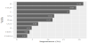
The most important parameters in the prediction of σRB are UCS and σh1, followed by depth and σv and finally by E and σh2 with relative importance levels below 10%. Figure 29 presents the importance of the variables for the SVM method. Equation 7 shows the relationship of the σRB model obtained by MR algorithm:
Considering the subordinate set of input parameters (group G2) the results slightly improve and the SVM model continues to have the best performance. In terms of importance, the main parameters are almost the same as in the previous case, namely UCS and σh1, followed by depth, σv and Q.
The DM techniques were applied to infer prediction models of the rockburst index IRB. For the Group G3 and considering all the tests, the model based on the ANN presents excellent results. The SVM model also gives good results, and the MR model showed the least accurate results. The relation between the input variables and the index IRB is highly non-linear which explains the excellent prediction of the ANN model. The most important variables are the depth and σRB followed by E, K and UCS. Equation 8 shows the obtained IRB relationship using MR algorithm for group G3.
Considering additional secondary variables, as was done for group G4, the same trends are observed in terms of the performance of the models. The most important variables are also H and σRB, followed by volume of the samples, Vol, and UCS and K. With reference to group G3 the performance of the models is quite different. The MR model presents the worst performance with considerably high error values, between 0.458 and 0.602 for a parameter with a mean value of 0.954 and ranging from 0.046 and 5.207. On the other hand, the ANN model presents excellent results shown by very low error values and an R coefficient very near to one. The SVM model also presents good results but it is clearly outperformed by the ANN model. For group G4, that considers also a secondary set of parameters, the results are similar to the previous case, although a slight decrease in the model’s performance is observed. In fact, the input parameters that were added to the process could not improve the model’s performance due to their low importance in relation to IRB. The only exception is the input parameter Vol.
6.2 In situ rockburst database and DM
In situ cases of rockburst that occurred during tunnel construction/ mining were collected from field studies at Jinping II, technical literature, publications and reports, and organized into a database. The rockburst cases were classified according to geometric characteristics, causes and consequences. DM techniques were then applied to the database with the aim of developing rockburst predictive models [92-93]. In order to understand the circumstances in which rockbursts occur, their magnitude, as well as the different consequences of rockburst, the authors gathered as much information as possible that could provide relevant information regarding the occurrence of the rockburst. For this, a form was created which included eight fields (each with one or more variables): (1) Occurrence of rockburst; (2) Method of construction; (3) Geometry of the tunnel; (4) Strength of the rock; (5) In situ state of stress; (6) Dimensions and location of the rockburst; (7) Severity and delay time; and (8) Damage in the tunnel. The database contains 60 cases, which is a relatively small number. However, we believe it constitutes a fundamental first step in order to create more complex models in the future. One important feature of the database is that most of the collected rockburst cases (91%) occurred during the construction of Jinping II. However, it should be stressed that the majority of rockbursts take place in deep underground mines. The collected data is confined to D&B and TBM excavation methods, and the shape of the tunnels where the rockburst cases occurred were circular (67%) and horseshoe (33%).
Different levels of rockburst were classified in accordance to Table 11, following the existing experience at the Jinping II hydroelectric scheme in China [4,10,41]. Figure 30 gives the distribution of cases in the database by rockburst type. In the figure overbreak situation corresponds to levels C and D.
Several DM techniques (DT, K-Nearest Neighbors, ANN and SVM) were applied to the database with the aim of developing rockburst predictive models. The R environment and rminer package developed by Cortez [84-85] were used for the implementation all DM techniques. For the prediction of in situ rockburst type a set of nine variables were considered, namely: L - Length of occurrence (m); TESC - Type of excavation; TSUP- Type of support; UCS - UCS (MPa); E - E (GPa); K - K0; FORM - Shape of tunnel; Deq - Equivalent diameter (m); Req - Equivalent radius (m).
The aim of the analysis was to develop models that would allow one to predict the type of rockburst given certain conditions and characteristics related to the underground work. For validation purposes a leave-one-out approach [94] was applied under 20 runs. For models evaluation and comparison, we used three classification metrics based on a confusion matrix [66].
Another outcome of the application of the DM techniques is the possibility of obtaining the importance of each of the model variables through sensitivity analysis [18]. According to the ANN model, the relevant variables are K, TSUP and L, with a total influence around 57% (Figure 31).
BN were also applied to the database [9,66]. The techniques used included Naïve Bayes Classifier, which are simple probabilistic classifiers based on Bayes Theorem, a particular class of BN with assumed independence between predictors; tree augmented Naïve Bayes Classifier, an extension of Naïve Bayes, where each attribute variable will have on parent variable between the other attributes, and Augmented Naïve Bayes (ANB), a semi-naïve structure. Several sensitivity studies were performed to determine the most influent variables in the prediction of rockburst type, which were found to be: (i) Support Type; (ii) K0; (iii) UCS; (iv) Deq; (v) Orientation (only for the Naïve Bayes and the TAN models; ORIENT means the orientation of the burst in the periphery of the excavation). The “best” BN classifiers are indicated in Figure 32.
The results of the different models were validated using 5-fold cross-validation method [94]. It was observed that the application of the TAN classifier results in a slighter improved classification then the other two models. This is expected as TAN has normally a better classification performance than standard Naïve Bayes. Naïve Bayes networks are a very simple representation of a problem, which can be an advantage, however the independence assumption, which is made in these models is many times incorrect and unrealistic. TAN are improved versions of Naïve Bayes networks which consider dependence between attributes in the models, which is normally more realistic than Naïve Bayes. The downside is that the process of adding dependencies between variables to capture correlations between the attributes, increases the computational complexity.
Confusion matrixes for the Bayes Naïve model and for the TAN (the lowest and highest accuracy of the “best” models) were calculated. It was observed that the Naïve Bayes model classifies all cases of Overbreak correctly. It also classifies 83% of Strong Rockburst correctly and 75% and 87.5% of the Moderate and Slight overbreaks correctly, respectively. The TAN model performs slightly better, classifying Overbreaks and Strong rockburst correctly on all cases. However the model, as with the Naïve Bayes model, cannot accurately classify all moderate and slight rockbursts, classifying correctly only 80% and 87.5% of these cases, respectively. This may be explained by the small number of cases in these two categories. In the future, extending the database will help improve the overall accuracy of the models.
7. Conclusion
The use of underground space for engineering systems has been increasing worldwide. Underground geoengineering is characterized by complex, uncertain geology and geomechanics that present challenges that require new techniques to be dealt with. Artificial Intelligence (AI) techniques provide a means to deal with these ever more complex and large data that are generated from the design and construction of these systems.
In this advanced review paper, the application of Data Mining (DM) techniques to deep underground engineering problems was discussed, and case studies were presented that illustrate the use of these techniques. Specifically, DM techniques used in the evaluation of geomechanical properties parameters in a large underground hydroelectric scheme, a very deep underground research laboratory, and to the prediction of rockbursts were illustrated. The models developed showed good accuracy with reality, and have the advantage to allow one to identify the importance of various parameters, as well as, in the case of BN classifiers, the relationship between these variables. The wide range of case studies shows, the importance that such AI techniques can play in future underground engineering problems. Novel studies are being developed to identify new strength criteria for rock mass in order to meet the demand of the scientific rock mechanics community.
Competing Interests
The authors declare that they have no competing interests.