1. Introduction

Most of the times, nature is unfriendly to us. Many times, nature seems to be really vindictive, humbling us with her power. The epitome of natural disaster is the earthquake, which can achieve a rate of released energy per unit time that surpasses any man-made or natural phenomenon with the exception of lightning.

All scientific and technological work is motivated by one of three pulsions: to exploit, to control or to predict nature.

The exploration of tectonic energies is still beyond the most optimistic scenarios. Control was ironically mentioned by Voltaire in the context of the great Lisbon earthquake: “It had been decided, by the University of Coimbra, that the spectacle of some people being slowly burnt, in a grand ceremony [an inquisitorial “auto-da-fé”], was an infallible way to prevent the Earth from shaking” [1]. More recent (and serious) attempts to control seismicity have been made but were always unsuccessful [2].

Earthquake prediction is, arguably, the ultimate drive that led to the earlier development of seismology.

In 1999 the online edition of Nature magazine held a debate, which was moderated by Ian Main [3], under the theme “Is the reliable prediction of individual earthquakes a realistic scientific goal?”

In that very educational debate, supporters and adversaries of earthquake prediction confronted their arguments and in the end, as would be expected, no definitive conclusions were reached that could change anyone’s opinions. The main outcome of this debate was a very strict definition of what rules must be universally accepted in order to verify the goodness of forecasts and forecasting methods.

2. Definitions

In [3] Main introduced what he called “a sliding scale of earthquake ‘prediction”:

1. Time-independent hazard [estimation], where seismicity is assumed to be a stochastic (Poisson) process. Prediction is only probabilistic.

2. Time-dependent hazard [estimation], where seismicity is assumed to be variant in time, but no random. This includes the seemingly contradictory concepts of “seismic gap” [4] and of earthquake 48 clustering [5] but also that of a characteristic earthquake that is approximately periodic [6]. In the present context, many people in Portugal are convinced that the “big ones” have a repeat period of about two hundred years which would mean that we are now “late”.

3. Earthquake forecasting, where forecasting is based on the monitoring of precursory phenomena, which [3] apparently restricts to physical precursors. The author says that this kind of prediction “would still be probabilistic, in the sense that the precise magnitude, time and location might not be given precisely or reliably (…) Forecasting would also have to include a precise statement of the probabilities and errors involved (…) The practical utility of this would be to enable the relevant authorities to prepare for an impending event (…)”.

4. Deterministic prediction, where earthquakes are assumed to be inherently predictable – seismicity would thus be a purely deterministic process – within very narrow time, magnitude and location windows.

   What will be discussed in the present work is Main’s concept 3, or “earthquake forecasting”. Main focuses on physical precursors but the concept can be extended to the analysis of time series of seismical parameters in earthquake catalogues assuming, which is common sense, that each earthquake is a precursor of the next one. It is well accepted today that seismicity is neither purely random (not even in time, since we know for centuries that it is not at all random in space) nor purely deterministic – it is a chaotic process and, most likely, one of self-organized criticality [7].

   This leads us to the definitions of foreshocks, main shock and aftershocks. These terms have been used too loosely, and it is common to read in the generic press that “an aftershock (or replica) can be stronger than the main shock”. This use has the social benefit of preparing the populations for a worst-case scenario, not neglecting vigilance after a strong earthquake, but is scientifically unsound. In an earthquake swarm, the strongest event is the main shock, those previous to it are foreshocks and those after it are aftershocks. Even so, recent work helped cast some additional confusion over these definitions: “main shocks are aftershocks of conditional foreshocks”… [8].

3. Sociology of Earthquake Forecasting

Earthquake forecasting has been a concern not only of seismologists but of the whole of society, from the everyday citizen to the large corporations (utilities, insurance companies).

The most cited successful prediction case was the Haicheng (People’s Republic of China) earthquake on February 4, 1975 (M=7.9). Prediction was based on the analysis of a foreshock swarm but also on Chinese traditional methods, which included the observation of abnormal animal (mostly snakes) behavior. Another successful prediction was later made by Chinese authorities for the August 16, 1976 (M=7.2) Songpan earthquake. Adversaries of prediction claim that these successful predictions were the only ones (as a matter of fact, the Songpan prediction is mostly forgotten), and that the same methods failed to 81 predict the Tangshan earthquake (July 27, 1976; M=7.6; more than 250,000 casualties).

Lore has it that hundreds of thousands of lives were spared by the timely evacuation of Haicheng province but these numbers don’t seem to be supported by documental sources [9].

A strong point remains, however, that even if a single human life was spared because of an accurate scientific prediction, this is ample justification for endeavoring in prediction research. This is also an argument in favor of a continuing publication of predictions, which is not the same as the issuing of occasional strong earthquake warnings. The social aspects of earthquake forecasting should be taken into account. Some authors (e.g. [10]) mention that the side effects of a prediction (panic, market falls, insurance rises) could be worse than the effects of the earthquake itself. This, however, has never happened, either in China, or in Japan (between1965 and 1967), or in the USA (1974, 1988, 1992). All these predictions proved to be false alarms and had no social consequences apart from a growing public and administration disbelief in earthquake prediction [9]. Since then, no formal “earthquake warnings” were issued by authorities, as far as the present author knows.

The prediction of another type of chaotic phenomenon – weather forecasts – has been around for decades and perhaps we can draw lessons from this application.

The argument that earthquake forecasting can cause widespread panic (which we saw is unlikely) has been surpassed by meteorology and climatology. Although the annual damages caused by weather are atleast one order of magnitude higher than those caused by earthquakes, short-range weather and long-range climate forecasts haven’t been known to cause social distress. This happens because meteorology has entered our everyday lives, helping us plan everything from vacations to crops and, furthermore, helping the authorities in large-scale planning.

Imagine, for a while, that weather forecasts were only issued prior to extreme weather phenomena. This could be both a cause for social insecurity or for apathy if, as in the case of earthquake forecasts, most predictions were wrong. Remember that, although short-term weather forecasts are very accurate, long-term weather forecasts are arguably not better than earthquake forecasts if seasonal effects are removed.

As [11] puts it, “(…) scientists have an even greater responsibility to communicate carefully their findings in earthquake prediction. By this, I do not mean keeping quiet about results. (…) Our obligation is to communicate our results in the clearest possible way, including when possible a statistical assessment of their validity. (…) Research should be separate from public policy, and the criteria for public use of earthquake information should be independent of the criteria for scientific study. (…) We cannot justify expenditures if we have not demonstrated that our assessment is better than random. This approach to public policy is independent of scientific research where we must continue the research into causal precursors both for our understanding of the physics of earthquakes and for any future hope of obtaining a predictive precursor.”

Some strong ideas arise from [11]:

1. Public accountability: the public is entitled to know how we spend their taxes.

2. Clarity in the dissemination of results, always including a probabilistic estimate of their validity.

3. Forecast quality should be measured against random probabilities.

4. Public policy should take into account the results (statistical, informational) of earthquake prediction research – albeit with different criteria than those governing research on physical precursors.

   Geller, a “forecasting skeptic”, puts forward another strong requirement [12], that

5. “(...) prediction proponents should, but do not, provide a ‘predictor in the box’ software package, with all parameters fixed. [Is there a meteorological ‘predictor in the box’?] (…)The software package would then generate predictions that could be tested against an intelligent null hypothesis”.

This work intends to address these five issues.

Cautious publication has been a concern of the present author. The forecasts that were made were always first published in specialized meetings and publications. However, on many occasions, the existence of a forecasting method and its simplified description were widely divulged to the generic media. The forecasts themselves weren’t because, until now, there was no clear, un-alarming way to make that divulgation. One of the main purposes of the present work was to try and find a way to make earth quake forecasts available to the public.

The proposed forecasting method should evolve into the periodical publication of seismic probability maps as those that are shown below. This will have two beneficial effects:

1. To get the general public acquainted with earthquake forecasting, its successes and failures, helping, at the same time, to divulge a much needed culture of responsible safety and preparedness.

2. To the authorities, since civil protection resources are always scarce, the knowledge of an increased probability of an earthquake occurrence could help cluster some of those resources on the most threatened areas during the windows of highest probability.

One area where scientists are not accountable is on the effect of their work on public policy – provided the authorities have knowledge of the forecasts that are eventually made. The results of the present work have been previously communicated to the Portuguese civil protection authorities, and will continue to be so.

The issues of the evaluation of forecast quality and of providing a “predictor-in-a-box” will be dealt with in the next paragraphs.

4. How to Evaluate the Quality of a Forecast

The theory of probability was developed mainly as a theory of gambling by French mathematicians of the 18th century. Even today, compulsive gamblers compile extensive statistics of the outcomes of their game of choice, in the chimerical hope to beat the odds. Was it Laplace who said that “lottery is a tax on the mathematically ignorant”? The underlying principle is that even a minute gain over the probability of a random event can be turned into a large profit. This principle cannot be applied to truly random processes which, by definition, have no memory, but is indeed applicable to the forecasting of processes with some memory, such as earthquakes: any method that yields better forecasts than a conventional statistical (Main’s type 1) analysis can be made to produce social benefits.

There are several statistical methods to evaluate the quality of a forecast. Of these, four will be described here [13].

Let there be A_i, any parameter of an actual earthquake, and F_i, the forecast that was made of the same parameter for the same earthquake, and N the number of (A_i, F_i) test pairs.

MAD= ∑ i=1 N | A i − F i | N (1)

Mean square error (MSE) is the average of the squared differences between actual and forecast, and the root mean square error (RMSE) is simply the square root of MSE:

MSE= ∑ i=1 N ( A i − F i ) 2 N (2)

RMSE= MSE (3)

Theil’s U-statistic (U) is much used in financial forecasting but less known outside this field:

U= MSE/ ∑ i=1 N A i 2 N (4)

It is intuitive that Pearson’s correlation coefficient (R), between actual and forecast series should be a good measure of the generic success of a forecasting method. However, R suffers from a limitation: it is not scale-independent.

R= Cov( A i , F i ) σ A σ F (5)

where is the co-variance between actual and forecasted parameters and and are the standard deviations of both sequences. Seismicity being a strongly nonlinear phenomenon, a very high absolute R is never to be expected.

5. NCEL: An Earthquake Predictor-in-a-box

Chaotic time-series arise in many fields, but one field in which their prediction is of everyday use is finance. A number of numeric tools was developed that enable technical analysts to forecast future trends in financial markets – the so-called “financial oscillators”. Time-series of earthquake parameters are also chaotic, often with comparable fractal dimensions, and testing the financial oscillators on seismicity was anatural step. The first applications of these tools for seismic prediction, though encouraging, had two shortcomings: first, their outputs are qualitative, since the oscillators only indicate if a trend is rising, declining or stable (“buy”, “sell” or “hold”); then, when several oscillators are applied to the same sequence the results are not always consistent. Both quantitative output and consistency were achieved by integrating the oscillators in an artificial neural network (ANN). ANN are software emulators of the nervous system and seemed adequate because of their mathematical universality, fault-tolerance, and ability to deal with semi-quantitative data such as the modified Mercalli intensity [14].

The oscillators that are used were described in detail in [14]. These are moving averages convergence-divergence, relative strength index, real-modulated index, optimized decision index, stochastic oscillator and momentum. Another tool was used originally, a very simple minimal-distance pattern recognition algorithm, but it was replaced in the present work as will be seen below.

The neural network architecture that was chosen is a partially connected, feed-forward, back propagation, three-layered perceptron. The neurons are arranged in one input layer, one middle, orhidden, layer and one output layer; neurons in each layer do not communicate among themselves, but only with those in adjacent layer (s); the weights of the connections between neurons are updated according the delta-rule [15].

The present author has been working for the past 15 years in the development of an earthquake forecasting method, with two successful forecasts in the Azores: the earthquakes of 1998.07.09 [16] and 2004.01.28 [17]. There were no false alarms.

The forecasting windows were still too wide and efforts were made to narrow them the most, within the limits of predictability of a chaotic phenomenon. In short, one will never be able to specify a day of occurrence.

Also, the geometric component of the input data and the forecasts was a semi-quantitative “location” parameter, not the usual latitudelongitude geographical co-ordinates. In the Azores this parameter was, earlier [16], the island “number”, east to west, and, later [17], the absolute value of longitude, in degrees.

Another shortcoming of the previous works was that an analysis of the forecast errors in the training sets was never much deepened: those errors were used only to empirically derive confidence intervals for the forecasts.

Recent efforts to develop the neural forecasting method were focused on

1. Narrowing the forecast windows;

2. Forecasting the geographical co-ordinates of the epicenter;

3. Quantitatively assessing the forecast errors;

4. Comparing the results of this method with those of other methods;

5. Automating the method the most, so that it can be used routinely by anyone with a minimum preparation.

These objectives were attained by integrating all prediction algorithms in a Microsoft™ Excel®workbook called NCEL.

The NCEL workbook consists of eight worksheets and one Visual Basic® (VB) module.

Worksheet “Cover” contains general instructions for use of the workbook.

Worksheet “Main” is the only one where the user can input data: a series of up to 1000 records of four earthquake parameters, event time and magnitude, epicentral latitude and longitude. It should be stressed that input data must have some sort of pre-processing. In all the examples below, the series were truncated for the lower magnitude events (non-linear bottom part of the Gutenberg-Richter function). Also, as a crude rule-of-thumb method to filter off foreshocks and aftershocks only the strongest earthquake in each day was used. The user can also, if willing, hand-tune most of the parameters of the neural network: length of the training set, number of neurons in the middle layer, learning rate, learning momentum, limit target error and limit number of iterations. However, default values for all these parameters are supplied. Namely, in the earlier works, the length of the middle layer vector was chosen so that the total number of connections was of the same order of the number of training examples.

In NCEL the default number of neurons in the middle layer is chosen according to the algorithm in [18] so that

j= me n+z (6)

Where j is the number of neurons in the middle layer, m is the number of training examples, e is the allowed error in percent, and n and z are the number of neurons in the input and output layers, respectively. It is also from a button on this worksheet that the neural network training is started. Worksheet “Oscillators” computes the financial oscillators for the input series. Also, the original pattern recognition algorithm was here replaced by the Excel function “TREND”, based on the previous twenty events.

Worksheet “Normalized” normalizes the input data and the oscillators in the [0,1] interval.

Worksheet “NN” de-normalizes the neural network outputs of VB module “NCEL” returning them in the familiar time-magnitudelatitude- longitude form.

Worksheet “Monte Carlo” performs Monte Carlo forecasts based on the input data on worksheet “Main” . Worksheet “Previous” performs naïve forecasts based on the input data on worksheet “Main” : it forecasts, for the next earthquake, exactly the same parameters that are recorded for the last one (which is a significantly successful method for weather forecasts for about half of the year). Worksheet “Averages”, another naïve approach (or maybe not so much, as will be seen below), forecasts, for the next event, the average for each parameter of all the previous events.

Worksheet “Error Analysis” calculates and compares the error parameters (see 4, above) for the four forecasting methods. After starting the neural network training process from sheet “Main” , the user is directed to this worksheet, where the train-test procedures evolution can be followed.

Visual Basic module “NCEL” performs the neural network training and testing procedures. The training procedure is based on the algorithm provided by [19]. In its earlier versions, “NCEL” followed closely the previous method, with the exception of forecasting the epicentral co-ordinates. Several test runs made over well known datasets showed unexpected results: many times the forecasts that were made by the “Averages” naïve method produced the smallest errors, mainly in MAD. In order to quantify this result and to further automate the forecasting procedure, the current version of VB module “NCEL” was all included in a loop that stops on one of two conditions: a command that is entered by the user or [MAD(NN) < MAD(Averages)] for the time parameter. Worksheet “Error Analysis” keeps track of the number of times that the neural network performs better than the “Averages” algorithm.

Error on the time-parameter was chosen as a stopping criterion because, intuitively, time is both the most important and the most difficult parameter to predict.

Why are the results not always the same? The “Previous” and “Averages” spreadsheets, once initially computed are, of course, invariant. Differences arise on each new calculation of spreadsheets “Monte Carlo” (because of the intrinsically quasi-random nature of the method) and “NN”. In the NN case, the differences occur because of the randomly initiated connections’ weights. However, unlike in “Monte Carlo” , the final results of different network runs never differ by more than 5% (on 300 tested cases).

The data-set that was used to test NCEL is based on two sources: [20] for earthquakes from January 1, 1852 until June 30, 1991 and [21] from July 1, 1991. These data were spatially filtered between coordinates 34⁰ and 44⁰ N latitudes, and 5⁰ and 15⁰ W longitudes. Then the data were further truncated for completeness at M=5.0, where M stands for the highest magnitude reported for each event. The final data- set consists of 118 events. The best results for NN forecasts after 100 runs of module NCEL are shown in table I, “best” meaning here the smallest MAD on times of pause, which was the NN stopping criterion. Several conclusions can be drawn from table 1.

Table 1: Best results for NN forecasts after 100 runs of NCEL.

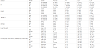
The scaling problems of R are obvious from a comparison of these parameters on dates and times of pause, which have exactly the same physical meaning but show very different R, meaninglessly always “good” for dates.

The NN has the best performance in all error parameters for pauses and latitudes.

The NN has the highest R for all forecast parameters. The values for pauses (0.512) and latitudes 284 (0.535) are significantly higher than the highest published value for tests of the earthquake forecasting 285 ability of neural networks, which was of 0.37 [22].

“Averages” has the best performance on MAD, U and RMSE for magnitudes and longitudes.

Globally, the neural network performs best on 88% of the parameters. Neither “Monte Carlo” nor “Previous” are ever the best forecaster; even so, “Previous” performs better than “Monte Carlo” on 65% of the parameters.

6. Presentation of Forecasts

As was seen above the present author believes that forecasts should be disseminated to the public. Publication should be, at the same time, scientifically correct and understandable by the widest possible audience. Presentation of forecasts in the form of probability confidence intervals around the point- forecasted values satisfy the former (scientifical correctness) but not the latter (clarity for the general public) as can be seen in table 2.

Table 2: Confidence intervals for NN forecasts.

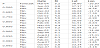
For example: the last two columns of table 2 shows the axes of confidence ellipses for several probabilities, P, for location of the epicenter of the next earthquake that was forecast by NCEL for continental Portugal. It is counter-intuitive that a higher probability should correspond to a wider area, as it does, and the same reasoning applies to magnitudes or dates. Publication in this form would be confusing. The authorities, however, should have access to this kind of tables.

It was found that the objective of making forecasts understandable by the widest possible audience can only be accomplished in the form of maps, much in the same way that other kind of forecasts, based on aftershock rates, are being presented daily by the United States Geological Survey [23]. Another problem arises from the use of magnitudes, which are not directly interpretable by the general public [23]. sensibly suggest that the reference should be made to a macro seismic intensity such as the modified Mercalli intensity (MMI) scale and that the forecast threshold should be put on MMI VI - “when objects are thrown off shelves, worst-quality masonry may crack and public alarm begins” [24].

This raises yet another problem: that of the magnitude-intensity conversion. Several magnitude-intensity conversion laws have been deduced and they are all of the form.

I=aM−blog(D)+c (7)

Where I is the intensity, M the magnitude (usually, MS – surfacewave magnitude), D the focal distance and a, b and c are empirically determined coefficients. For the present work, the chosen conversion law was that of [25], with a=1.5, b=5.0, and c=6.0. MS is being systematically reported only in recent years, so the magnitude that was used was the largest reported for each event. Small changes in a, b and c in equation (7), do not affect significantly the output, which will have the form of a color gradation map.

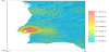
The map for daily background probability of occurrence of an earthquake with I ≥VI was built in the following way:

1. The study area was binned with a 0.1⁰ 0.1⁰ grid;

2. For each of the 118 events in the working data-set intensity was calculated on each of the bins;

3. A separate array stored the number of times, Ni, that I ≥VI was reached on bin i;

4. Dividing each of the final Ni by the total number of days that the dataset spans, yields Pi, the daily probability that an earthquake will be felt with I ≥VI on bin i.

Probabilities were mapped to produce figure 1.

Figure 1: Background daily probability of feeling an earthquake with I ≥VI.

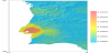
To produce a probability map that incorporates both background and NCEL forecast information, the confidence interval ellipse for P=0.5 was used (see table 2). For each 0.1º 0.1º bin the highest probability was chosen (background or forecast), and plotted (figure 2).

Figure 2: Forecast daily probability of feeling an earthquake with I ≥VI.

7. Conclusion

Averages – the calculation of recurrence periods – is a simple, straightforward, forecasting method that should continue to be used to make general planning and engineering decisions. However, it is out performed by the neural network.

The neural network is not some sort of “black box” into which we feed data and from which predictions are produced. It is simply an algorithm that allows to detect otherwise hidden patterns in the data, and could possibly be replaced by a multiple regression algorithm. The advantages of the neural network are that it is computationally lighter (multiple regression requirements grow exponentially with the number of degrees of freedom) and fault-tolerant: there are sometimes large errors in the determination of earthquake parameters, especially in older events.

The method that was shown above can produce forecasts every time that there is a new earthquake. Those forecasts can, and should, be conveyed to the authorities in order to help rationalize scarce resources by assigning more of them to the most threatened areas during the windows of highest probability. Also the general public can benefit from the periodical publication of maps such as those that were shown here. Not only because the public has the right to know but also because they can, if informed, influence the authorities to produce better legislation and planning.