2.1 Representation learning

Representation learning is a method for obtaining valuable representations for classification and other purposes through self-supervised learning.

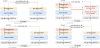
The major representation learning methods, such as SimCLR [7], BYOL [8], and SimSiam [9], share a common approach. First, x₁, x₂ are obtained by applying two data augmentations to a sample x. Second, z₁, z₂, that is, feature representations corresponding to x₁, x₂, are obtained from the neural network. Finally, the neural network learns to make the two obtained feature representations z₁, z₂ consistent. To achieve this policy, each method adopts a different method for the network and loss functions.

SimCLR (Figure 1a) is one of the earliest of these methods and is trained via the following algorithm.

Figure 1: Learning architecture of each Siamese Learning.

$\begin{array}{l}{x}_1,x_2=\text{aug}(x),\text{aug}(x)\\ z_1,z_2=g_{\theta }(f_{\theta }(x_1)),g_{\theta }(f_{\theta }(x_2))\\ loss=D_{simclr}(z_1,z_2)+D_{simclr}(z_1+z_2)\end{array}$

where D_simclr(z₁, z₂) is defined in Equation 1.

$-{\displaystyle \sum _{i=1}^N\log \frac{\exp (\text{sim}(z_{i1,}{z}_{i2}))}{{\displaystyle {\sum }_{j\ne i}^N{\displaystyle {\sum }_{k\in [1,2]}\exp (\text{sim}(z_{i1,}{z}_{i2}))}}}}$ (1)

Here, aug denotes random data augmentation, and sim denotes the cosine similarity. In addition, f_θ is a neural network such as ResNet [3] without the classification layer, and g_θ is a neural network consisting of one to three layers.

BYOL (Figure 1b) is an advanced version of SimCLR and MoCo [10]. There are two significant changes from SimCLR. The first change is ξ, which is the model parameter θ updated by a moving average, as proposed by MoCo. This implies that instead of predicting each z directly, prediction of z' output is learned using the model parameter ξ. The second change is to add a network h_θ to predict z and train the output p to predict z'. The algorithm is as follows:

$\begin{array}{l}{x}_1,x_2=\text{aug}(x),\text{aug}(x)\\ z_1,z_2=g_{\theta }(f_{\theta }(x_1)),g_{\theta }(f_{\theta }(x_2))\\ z_1^{\text{'}},z_2^{\text{'}}=g_{\xi }(f_{\xi }(x_1)),g_{\xi }(f_{\xi }(x_2))\\ p_1,p_2=h_{\theta }(z_1),h_{\theta }(z_2)\\ loss=\text{sim}(p_1,\text{sg}(z_2^{\text{'}}))+\text{sim}(p_2,\text{sg}(z_1^{\text{'}})),\end{array}$

Here, sg denotes the stop gradient.

SimSiam (Figure 1c) is a simpler version of BYOL and can achieve the same or better accuracy. Instead of using the moving average model parameter ξ introduced in MoCo and BYOL, p learns to predict each other’s z.

$\begin{array}{l}{x}_1,x_2=\text{aug}(x),\text{aug}(x)\\ z_1,z_2=g_{\theta }(f_{\theta }(x_1)),g_{\theta }(f_{\theta }(x_2))\\ p_1,p_2=h(z_1),h(z_2)\\ loss=\text{sim}(p_1,\text{sg}(z_2))+\text{sim}(p_2,\text{sg}(z_1)),\end{array}$

This simple method learns representations that are useful for classification.

Surprisingly, BYOL and SimSiam, which remove the explicit contrastive loss, produce different representations for each sample. This result is because of implicit contrastive learning by batch normalization [11].

2.2 Out-of-Distribution by Distribution shifting transformations

OOD detection aims to obtain a measure that distinguishes between samples included in the category of the training data and samples that are not. Rot [12] is an OOD detection method that uses self-supervised learning approaches. This method provides a sample of an image with four different rotations (0°, 90°, 180°, and 270°) and allows the neural network to predict the angle. This is because neural networks can predict the angle of rotation for images of the classes included in the training data, but not for other classes’ images. To infer the angle information, it is necessary to capture not only the texture but also the shape.

CSI [6] is a method that combines contrastive learning and distribution-shifting transformations. Distribution-shifting transformations are augmentations that shift the data distribution in N ways. The model learns each feature from the N new samples applied to a single sample as another sample. CSI also has a neural network that can predict the type of shift applied in N. In CIFAR-10, as well as Rot, the most accurate distribution-shifting transformations are the four types of rotations (0°, 90°, 180,°and 270°). CSI constructs representation learning from SimCLR [7] as contrastive learning. In other words, CSI combines SimCLR and Rot. Thus, the model embeds the angle and sample information in detail.

CSI also defines the OOD detection score S_con(x, {x_m}) for sample x in Equation 2, where z is a feature representation, and g_θ(f_θ(x)) and {z_m} are the feature representations of the training data set {x_m}.

$S_{con}(x;\{x_m\})=\underset{m}{\max }sim(z,z_m)\Vert z\Vert$ (2)

The smaller the detection score, the higher is the probability that the sample is an OOD sample. This score means that in-distribution features have a higher similarity to the feature representations of the sample in the training data, and OOD features have a lower similarity. However, because the OOD sample is assigned to a random feature representation, it may be similar to the feature representation in the sample. To avoid this problem, the detection score is the similarity multiplied by the norm of z, because the norm of f z is smaller when it is a random feature representation.

The detection score S_con−SI, which integrates S_con−SI obtained from each rotated sample xⁱ, is expressed by the following equation 3.

$S_{\text{con-SI}}(x;\{x_m\})={\displaystyle \sum _{i=1}^4{\lambda }_i^{\text{con}}{S}_{\text{con}}(x^i;\{x_m\})}$ (3)

Here, zⁱ is the feature representation extracted from the i-th rotation-applied to sample xⁱ, and the weights calculated from the training data are ${\lambda }_i^{\text{con}}=N/{\displaystyle {\sum }_m^N\Vert z_m^i\Vert }$ .

Furthermore, the metric S_cls−SI is defined using the output $r_{\theta }^i(f_{\theta }(x^i))$ for the rotated i-th angle obtained from the rot predictor r_θ. This score is represented by the weights ${\lambda }_i^{\text{cls}}=N/{\displaystyle \sum _m^N{r}_{\theta }^i(f_{\theta }(x^i))}$ calculated from the training data, as in Equation 4

$S_{\text{cls-SI}}(x)={\displaystyle \sum _{i=0}^4{\lambda }_i^{\text{cls}}{r}_{\theta }^i(f_{\theta }(x^i))}$ (4)

The final OOD detection score S_CSI in CSI was calculated from S_con−SI and S_cls−SI, as in Equation 5.

$S_{\text{CSI}}(x;\{x_m\})=S_{\text{con-SI}}(x;\{x_m\})+S_{\text{cls-SI}}(x)$ (5)

A previous study compared these indices and showed that S_CSI is the best OOD detection score.

2.3 AugMix with Jensen–Shannon divergence consistency loss

AugMix [13] is a method for data augmentation. This can improve the robustness and uncertainty of the model. As a feature, this method adds the Jensen–Shannon divergence (JSD) consistency loss to the loss function. This loss constrains the distance between each output probability distribution to be small when images to which the two types of data augmentation are applied, and the original image is input. The following loss function definesthis loss:

$\begin{array}{l}{x}_1,x_2=\text{aug}(x),\text{aug}(x)\\ y,y_1,y_2=P_{\theta }(x|l),P_{\theta }(x_1|l),P_{\theta }(x_2|l)\\ M=\frac{1}{3}(y+y_1+y_2)\\ JSD=\frac{1}{3}(\text{KL}(y|M),\text{KL}(y_1|M),\text{KL}(y_2|M))\end{array}$

where KL is the Kullback–Leibler divergence.

Adding the above loss function to cross entropy loss, the model learns to have probability distributions close to the original image, even when applying data augmentation. This loss function is also robust to noise that is not included in the data augmentation during training.

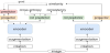
3.1 Contrastive learning like SimSiam

SimSiam [9] is a representation learning method that differs from SimCLR, mainly in the following three aspects:

1. projector composed of multiple layers;
2. adding a network to predict each other’s feature representation; and
3. implicit contrastive learning.

Because of these differences, SimSiam can perform representation learning with a higher accuracy than Sim- CLR, as described in related works.

SimSiam projects different samples to different representations without explicit contrastive learning because of batch normalization[11] in the network. In addition, implicit contrastive learning means that there is no need to constrain the different samples represented differently by a loss function since the final classification falls into some categories. The classification accuracy is high, even if images of the same class have highly similar feature representations.

In contrast, in good detection, matching all representations to the central representation of each class may lead to overlearning. This problem arises because learning features representing in-distribution well are quite different from learning features representing outof-distribution. Therefore, it is necessary to test whether explicit contrastive learning or implicit contrastive learning is better in such situations.

3.2 JSD consistency loss

Training with a rot predictor reduces representation learning performance, because cross entropy loss ignores the consistency of the feature representation until the probability distribution is completely sharp. However, the ideal probability distribution output is not one-hot, and the probability distributions between similar samples need to be closer than those between different samples. The usual cross entropy cannot learn such a consistency. To solve this problem, we introduce the loss function such that the expressions of the probability distributions y₁, y₂ that predict the rotation angles of x₁, x₂ are consistent. In this study, we adopted AugMix [13] and introduced the following JSD: suppose the one-hot distribution of the correct value of the rotation angle yt, the distribution of the predicted probability of the rotation angle y₁, y₂, and the mean of the three distributions M.

The JSD consistency loss is represented by Equation 6.

$JSD=\frac{1}{2}(\text{KL}(y_1|M),\text{KL}(y_2|M))$ (6)

As in AugMix, this loss function reduces overoptimization for cross entropy, which interferes with representation learning and encourages feature representations to match between x₁, x₂ in the process of learning consistency. Whereas AugMix is constrained using the distribution y obtained from the original image, our As in AugMix, this loss function reduces overoptimization for cross entropy, which interferes with representation learning and encourages feature representations to match between x₁, x₂ in the process of learning consistency. Whereas AugMix is constrained using the distribution y obtained from the original image, our method calculates the loss function using the correct answer value. This loss is multiplied by 12, similar to AugMix, and added to the cross entropy.

4.1 Dataset

We set CIFAR-10 as the training dataset, and the following seven datasets as the OOD: SVHN, LSUN, ImageNet, CIFAR-100 and Interp. OOD datasets are equivalent to the experimental condition of Unlabelled CIFAR-10 in CSI [6]; however, this study regards LSUN(FIX) and ImageNet(FIX) in the previous paper as LSUN and ImageNet.

4.2 Contrastive learning

SimSiam [9] and SimCLRs were used as the experimental targets for the contrastive learning method. The hyperparameters of SimSiam, such as architecture, data augmentation, and learning rate, follow those shown in previous studies. In addition, SimCLRs shares all the hyperparameters with SimSiam, except for the loss function, as shown in Figure 1d. However, the loss function is represented by D_simclr. SimCLRs follows the following algorithm:

$\begin{array}{l}{x}_1,x_2=\text{aug}(x),\text{aug}(x)\\ z_1,z_2=g_{\theta }(f_{\theta }(x_1)),g_{\theta }(f_{\theta }(x_2))\\ z_1^{\text{'}},z_2^{\text{'}}=g_{\xi }(f_{\xi }(x_1)),g_{\xi }(f_{\xi }(x_2))\\ p_1,p_2=h_{\theta }(z_1)h_{\theta }(z_2)\\ loss=D_{simclr}((p_1,\text{sg}(z_2^{\text{'}}))+D_{simclr}(p_2,\text{sg}(z_1^{\text{'}}))\end{array}$

4.3 Contrastive learning

We showed that the addition of a rotation angle prediction network, the rot predictor, degrades the performance of representation learning in the previous method. We also demonstrated that the incorporation of JSD consistency loss in training the rot predictor improves the performance of representation learning. To highlight these results, we compared the following four types of methods.

• w/o rot
• w/ rot, w/o rot predictor
• w/ rot, w/ rot predictor, w/o JSD consistency loss
• w/ rot, w/ rot predictor, w/o JSD consistency loss

The first is the baseline, which is used when OOD detection is not required. The second method trains images with four different rotations. The four rotations quadruple the batch size; therefore, the batch size of the original image should be 1/4. The third method is the same as CSI, which is trained with the rot predictor. In this case, the total loss is the sum of the similarity loss for representation learning and the cross entropy loss for learning the rot predictor. Finally, we added the proposed JSD loss to the third one during training.

4.4 OOD detection score with JSD

In this experiment, we adopted S_con−SI, represented by the expression 3 as the OOD detection score in the proposed method, that is, CSI with JSD consistency loss. The OOD detection scores of the comparison targets correspond to those of the original CSI, as shown in Table 1.

Table 1: Correspondence between presence/absence of each method and OOD detection score.

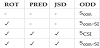
ROT denotes the presence of rotation augmentation, PRED denotes the presence of a rotation predictor, and JSD denotes the presence of a JSD consistency loss.

4.5 Parameters

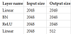
ResNet18 [3] was used as the neural network f_θ to extract the features. In addition, in both SimCLRs and Sim-Siam, according to [9], the projector g_θ is constructedas shown in Table 2, and the predictor h_θ, as shown in Table 3.

Table 2: Projector.

Table 3: Predictor.

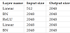
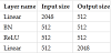
The original SimCLR does not have a predictor network, and the projector network consists of a single layer with an input size of 512 and an output size of 2048.

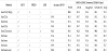
In this study, the rot predictor was constructed as shown in Table 4.

Table 4: Rot predictor.

The rot predictor in the original CSI is composed of a single layer.

6.1 Consistency loss for rotation predictor

The experimental results clearly indicate that training the rot predictor with a cross entropy without the JSD consistency loss reduces the classification accuracy. In particular, the classification accuracy was lower than that without the rot predictor. Thus, OOD detection by conventional CSI has a trade-off relationship with the classification.

Adding the JSD consistency loss addresses this tradeoff and improves the accuracy of OOD detection and the classification accuracy for the original contrastive learning. This result was not just because they suppressed the cross entropy. It is possible to learn better intermediate representations (i.e., feature representations) by introducing a loss function such that the probability distributions of image samples from the same image at the exact angle match.

6.2 Detection score with JSD consistency loss

In our experiments, S_con−SI, which is represented by Equation 3, is adopted as the OOD detection score in the proposed method. The reason for using S_con−SI instead of SCSI is that the introduction of this loss improves the accuracy of OOD AUROC, compared to using S_cls−SI in combination. This is because the accuracy of representation learning is improved. However, this loss reduces the angle prediction accuracy of the rot predictor. Therefore, the accuracy of S_cls−SI and S_CSI decreased compared to the accuracy without the JSD consistency loss.

6.3 Contrastive learning method for accuracy

As shown in the experimental results, regular SimSiam is more accurate than SimCLRs for unsupervised class classification using representation learning. On the other hand, when rotation augmentation is applied, SimSiam accuracy is lower. This is probably because the rotated images should be treated as separate samples, but they have very close feature values. In SimCLRs, the feature representations of the images in a batch are explicitly specified to be different; therefore, even if they are initially from the same samples, they are learned to have different representations for each rotated sample. In contrast, SimSiam implicitly performs contrastive learning through normalization. Therefore, if the image representations are genuinely close, they can be the same even after normalization. Because the rotated images are close to each other, it is difficult to determine whether they should be closer or further away from other data augmentation methods. It is assumed that this conflicts with cross entropy learning for separation and reduces the accuracy.

In contrast, there is little difference in the absolute accuracy when adding the JSD consistency loss. Cross entropy prevented the learning of feature representations from conflicting with the learning of feature representations, thereby moderating the intense conflicts that occurred, especially in SimSiam. Moreover, the model learns the feature representation through the predictive distribution of the rotation angle.

It is demonstrated that the final accuracy is affected by providing data whose distribution within a batch differs significantly from that of regular representation learning. The proposed method, with the JSD consistency loss, reduces this effect.

6.4 Contrastive learning method for OOD-detection

For regular classification applications, SimSiam [9] outperformed the original SimCLR [7] and SimCLRs. In contrast, in OODDetection, different results were obtained for different tasks. SVHN has a very high AUROC of 99.9% in the original CSI. However, even Sim-Siam + CSI + JSD, which is the best of the proposed methods, achieves 99.2%, which is lower than the original CSI. In addition, the accuracy is not consistent between SimCLRs and SimSiam. Furthermore, in Interp, which is a dataset of two blended images from CIFAR-10, the accuracy is inconsistent between SimCLRs and SimSiam. These datasets are considered to be more affected by the contrastive learning method than the others.