1. Introduction

Scheduling in manufacturing is an area that has interested researchers for at least the past 60 years [2]. It is the process of generating a plan (a schedule) that shows the order in which tasks are to be executed in order to achieve a purpose [3]. Together with planning, it lies at the heart of important decision processes in manufacturing companies.

These processes affect the central operations of the company, including procurement, production, distribution, transportation, information processing and communication [2]. Maximising productive manufacturing time is essential for the manufacturing industry to maintain profitability [4]. This requires efficient utilisation of resources as outlined by Edgett in his article for Manufacturing.net, a leading web site with up-to-date information about manufacturing [5]. And better scheduling ensures the best employment of available resources.

There is an outstanding amount of research related to scheduling problems. Blazewicz et al. define scheduling problems as the problem of allocating resources over time to perform a set of tasks that make up a larger process [6]. Individual tasks compete for resources and tasks can have relations between them affecting the way in which they can be processed.

Today, the manufacturing industry is facing very difficult market conditions that force it to strive for efficiency besides guaranteeing quality. This has given rise to the term Lean Manufacturing. This is a production control technique that aims at eradicating inefficiencies from the manufacturing process. There are a number of techniques that build on this philosophy, namely the Toyota Production System, Just-In-Time (JIT) Manufacturing, Kanban and 5S [7].

Scheduling theory deals with different problem types, and a large volume of literature, models and approaches that describe and attempt to solve different scheduling problems. Scheduling theory uses information already at hand at the manufacturing plant to find a feasible schedule for the manufacturing operations to be executed on/by the required resources. This information includes, but it is not limited to, the type and amount of each resource used in the manufacturing process, the sequence of the tasks necessary to manufacture an item and the time required for each task [3].

2. The purpose and scope of this study

This study was part of a two-year research project financed by the European Regional Development Fund (ERDF) called Research Services in Manufacturing: ICT in Manufacturing. The objective of this process was to create a software solution that allows operators to model production lines and determine and classify the scheduling problems represented by the model.

It has long been felt that not enough information is available regarding the scheduling problems affecting the manufacturing industry in Malta. This project was undertaken to gain additional information on the state of scheduling in the local manufacturing industry and to provide an extensible framework that can be used for current analysis and future research.

This study focused on providing a graphical means of representing scheduling problems. This representation describes the abstraction of the production line involved in manufacturing a product. The second aim of the study is to create a set of heuristics using the model to classify the scheduling problem according to its computational complexity, and when possible, pointing to the relevant literature used to derive the classification in order to help researchers understand the problem better.

Scheduling involves efficient utilisation of scarce resources. While this study focuses on scheduling in manufacturing industry, Leung draws a parallel to the problems encountered by computer scientists in the 1960s when computational resources (CPU, memory and I/O devices) were scarce [8]. This results of this study are of interest to computer scientists, operators in the manufacturing industry whose work deals with scheduling and to researchers in the field of optimisation.

3. Production Line Graph Modelling

Graphs are a flexible mathematical structure that are used for representing a wide variety of problems. In particular, they are useful for representing relationships between abstract entities. Bondy and Murty, in fact, note that many real-world situations can be modelled using graphs [9].

Bondy and Murty define a graph G as an ordered pair (V(G), E(G)) consisting of a set V(G) of vertices (or nodes) and a set E(G) disjoint from V(G), of edges with an incidence function ϕG that associates with each edge of G an unordered pair of vertices of G [9]. If e is an edge and u and v are vertices such that ϕ_G(e) = {u, v} then e is said to join u and v. u and v are called the ends of e. The number of vertices in G is denoted by v(G) and the number of edges is denoted by e(G). v(G) and e(G) are referred to as the order and the size of G respectively [9].

Graphs have been used in many of areas of computer science. For instance, Heller and Schneiderman describe how data structures can be modelled using graph theoretic principles [10]. Their paper describes how graph-based data structures can be used in databases for organising records supporting the search for data in a given field or a subset of fields. Mirza has used a graph theoretic modelling approach to link content in a recommender system [11]. The aim of the algorithm was to use graph theory to identify links between entities in a social network. Caramuta used a graph-theoretic approach to Decision Theory in order to explicitly represent memory when individuals make choices [12].

There are several examples of how a graph-theoretic model has been employed to represent aspects of scheduling problems. Sanmarti et al. use a graph representation called the S-Graph for specifying specific chemical processes in multipurpose batch plants [13,14]. Their approach demonstrates how graphs are well suited for modelling complex scenarios as in this case they model a flexible environment where the number of products is very large and where alternative paths may be used to manufacture the same product.

A second technique described by Friedler and Fan for modelling a manufacturing process is the P-Graph [15]. Also known as the Process Graph, this is a bipartite representation of the structure of a process system. Operating units in P-Graph are represented by horizontal bars while input and output materials are represented by solid circles. The direction of the edges of the P-graph indicate the flow of material in the network. Operating units cannot be connected, and therefore, there cannot be any edges between horizontal lines.

P-graphs were designed to overcome problems in graph-based approaches depending on directed graphs or signal flow graphs. In digraph modelling, operating units correspond to vertices while connections are represented by edges of the graph. In signal-flow graphs, vertices represent the materials of the process. While these models excel at representing and analysing the system, they fail to adequately describe process synthesis. The sleek form of the P-graph captures the syntactic and semantic contents of the process structure.

Two other graph representations that have been considered are the Resource-Task Network (RTN) and the State Task Network (STN). The first was developed by Pantelides and is a unified framework that is used in the description and solution of a variety of process scheduling problems [16]. TRTN is based on bipartite graphs, and is made of two nodes:

1. Asks: A task is an operation that transforms a certain set of resources into another set.
2. Resources: A resource includes all entities that are involved in the process such as materials, processing and storage equipment, utilities and setup conditions.

The State-Task Network (STN) is a scheduling model that is used in multi-product batch plants and that can be applied to batch processes that are specified by recipes. It is used in short-term scheduling where demands for products are specified by deadlines [17]. The capabilities of STN are:

1. The model does not require a fixed assignment of equipment to process tasks;
2. Batches are variable-sized, and can be mixed and split;
3. The model supports different intermediate storage and transfer policies as well as limitations of resources.

4. Defining Scheduling Problems

Formal models based on this information allow researchers to define and understand scheduling problems and then search for optimal solutions. These models are required to remove ambiguity, to arrive at an improved descriptive precision [18]. Such methods allow for consistency, analysis and validation, thus ensuring correctness. They can be used for working out the consequences of particular constraints, and also help to identify the effects of possible changes.

We refer to the notation by Graham et al. to describe a scheduling problem [19]. This notation is widely used in literature and should provide a coherent platform for discussing the composition of scheduling problems. In summary, this notation describes scheduling problems using three fields, namely α, β and γ described hereunder:

α refers to the machine environment and is made up of two fields, α₁ and α2. α1 represents the machine environment and can be an element of {ε, P, Q, R, F, J, O}. The following list describes the different values that can be used in each of the fields:

1. α₁ = there is a single machine,
2. α₁ = P the machine environment consists of identical machines,
3. α₁ = Q the machine environment consists of uniform machines,
4. α₁ = R the machine environment consists of unrelated machines
5. α₁ = F a flow shop represents a problem in which jobs have one operation for each machine such that all machines are used in the same order;
6. α₁ = J a job shop is a problem where each operation is ordered according to some manufacturing plan;
7. α₁ = O a open shop is a problem where there are no constraints on operation processing.

α₂ represents the number of machines (given as a positive integer). This field can store the values {ε; 1, 2, 3, 4, 5, m}. α₂ can be 1 only if α₁ = ε. When α₂ = ε, there is a variable number of machines.

β= {β₁; β₂; β₃; β₄; β₅; β₆; β₇; β₈} represent the job constraints of the scheduling problem.

1. β₁ ε {pmtn; ε} - This field represents job-splitting or pre-emption;
2. β₂ ε {res; res1; ε}- This field represents resource constraints that are required for the manufacturing of a job;
3. β₃ ε {prec; tree; chains; ε}- Jobs may have precedence constraints defined on them, such that if a job depends on another it cannot start unless the job it depends on has been manufactured;
4. β₄ ε {r_j; ε}- Jobs may have release dates, which are represented in these fields;
5. β 5 ε{ mj≤ m ¯ ; ε } - Defines a ceiling on the performance of a machine’s ability to manufacture the job;
6. β₆ ε {p_i = 1; p_i = p; p_{i j} = 1; p_{i j} = p; ε}- Represent the processing times it takes to manufacture the job;
7. β₇ ε {d_j; ε}- Jobs may have deadlines which are end dates beyond which the job cannot be manufactured;
8. β₈ ε {no-wait; ε}- This field is present in Flow Shops, where no buffers are present and jobs are started in succession;
9. β₉ ε {s-batch; p-batch; ε}- Represents a batching problem, a problem where jobs are manufactured jointly on one machine.

The optimality criteria for a schedule is given by γ∈{ f max , ∑ f j } and it represents the function to optimise. For a schedule s, we can compute for each job J_j :

the completion time or makespan C_j : the amount of time required to complete a pre-identified group of jobs;

the lateness L_j = C_j-d_j : the difference between a job’s completion date and it due date;

the tardiness T_j = max{0;C_j-d_j}: the amount of time it takes to complete a job once its due date has passed, otherwise 0;

the earliness E_J = max{0; d_j-C_J}: the amount of time until a job’s due date arrives once the job has been completed; or

the unit penalty U_j = if C_J ≤ d_j , then 0 else 1: assign a penalty if the job was manufactured earlier than the due date.

Thus, the optimality criterion seeks to minimise f max ∈{ C max , L max } where f max = max j { f j ( c j ) } with f_j(C_j)=C_j, L_j or ∑ f j ∈{ ∑ C j , ∑ T j , ∑ U j , ∑ w j C j , ∑ w j C j , ∑ w j T j , ∑ w j U j , }

The optimal value of γ will be denoted by γ^* which is the value produced by an approximation algorithm A for γ(A).

5. Classification of Scheduling Problem

The classification of scheduling problems is done through a tool which classifies scheduling problems by matching them against a database of known results. The results are published and maintained by Knust and Brucker and include a set of digraphs that represent a reduction that are used to determine if one problem is related to another [20]. The principle of the classification engine is based on the model proposed by Lageweg et al [21,22]. An online version of the tool was developed by Dürr [23].

Lageweg et al distinguish between “easy” and “hard” problem types by specifying that an “easy” problem is a problem for which there exists a polynomial time algorithm [21]. A “hard” problem is a problem which is known to be NP-Hard. MSPCLASS, the program they came up with, maintained a list of problems known as “easy” and “hard” problems. It then, systematically, employs a partial ordering to derive the status of the individual problem and to classify the problems as open, easy or hard. Moreover, it can also determine the following subclasses of problems, namely:

1. maximal easy problems;
2. minimal open problems;
3. maximal open problems;
4. maximal hard problems.

A particular problem may belong to different categories if its word list is a subset of the words of more than one category. The universe of a category is constructed using the union of the words in the components that are associated with the category [20]. A component is a directed acyclic graph whose nodes are word sets. The set of nodes of the DAG are the domain of the component. These components are the basic block of the reduction rules that the classification engine uses to deduce whether a problem is an instance of another. The union of the word sets of the components (which can belong to just one category) make up the universe of that category [20].

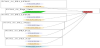
The graph of a component is connected and its transitive closure defines a partial order which specifies the rules to use to deduce the relationship between a particular problem and another problem in the database. The partial order is only valid within a certain context, which is the category. Figure 1 shows the reduction graph for γ , which is common to all categories. The comparison is only done when a problem falls within one of the components defined by the engine. Problems from different categories cannot be compared. If there is a category such that for every component in the category one problem Π₁ has smaller or equal values than problem Π₂ according to the partial order, then Π₁ is a particular case of Π₂.

Figure 1: Reductions for γ, applying to all categories.

To determine the category of a problem, the classification engine finds the intersection of the category’s universe with the word set of the problem. If the result is that the problem’s word set is in the universe of the problem, and it has a value for every component associated with the category, then the problem belongs to the category. This allows the classification engine to determine which problems can be matched to the problem being classified [21].

The classification engine was developed in T-SQL on Microsoft SQL Server 2008 R2. The following are the rules that are used to determine whether one problem is a special case or a generalisation of another problem. The basic component of the classification engine is the category. A category represents a collection of problems, and it is defined as the collection of words that describe the collection of problems. Words are the elements that make up the signature of a problem. For example, considering 1|pmtn; r_i| _Cmax as an example, the words for this signature would be 1, pmtn, r_i and C_max. The union of the words in a category is called the universe of the category.

5.1 Approach

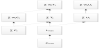
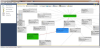
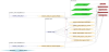
The approach adopted in this study was to create a system whereby a user can “translate” a physical model into an appropriate abstraction that can be used by a computer to detect and classify scheduling problems. Figure 2 describes the process. The signatures were generated using the Graham et al notation are able to describe specific scheduling problems as well as classes of scheduling problems which are useful for classifying scheduling problems [19].

Figure 2: Graphical Representation of the Approach.

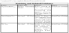
While the approach is good for a short technical description of a scheduling problem, it requires a good knowledge of the notation and know-how in analysing manufacturing shops and production lines. Our approach to model production lines builds upon the notation but uses a graph to describe the interactions between the different components. The nodes used are specified in table 1.

Table 1: Node Representation.

Each graph node represents an entity of the α|β|γ representation. An additional node represents information about the model. The model allows lines to be associated to different shops, as is the case in most manufacturing establishments. It is common terminology in manufacturing environments to refer to areas of a factory where manufacturing takes places as a shop floor.

A processor is a unit of manufacturing that is used to produce a product or a component. A processor is available to just one shop and may represent a single machine or a set of (parallel) machines. In accordance to the definitions proposed by [19], we distinguish between identical, uniform and unrelated parallel machines and further specify if the machines are multi-purpose machines.

Manufacturing jobs are not limited to be manufactured in a single shop. The operations (or tasks) of a job may be processed by machines in different shops. Hence a job represents the product that it related to and the operations represent the tasks that are required to produce the item. A job node gives information on the processing time of the job and gives details on whether the job has deadlines or release dates associated with it.

Job operations are associated primarily with the job to which they are related, and the machine(s) where they will be executed. Associated with the operation, there is also the individual processing time (which contributes to the total processing time of the job) and whether the job can be split after the operation has been completed. It is assumed that a job’s operation is atomic,and that job splitting is permitted only after a whole operation has been concluded.

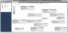
Figure 3 is an example of a simple production line used to test the modelling of a production line. Each node visually shows the information about the entity it represents. Internally, the node stores an entity object that contains a copy of the data that defines it. The model is persisted to the back-end database so that it can be reused. Table 1 provides a list of the information stored in each node type.

Figure 3: A complete model represented as a graph.

6. Evaluation

The evaluation was carried out in conjunction with local industry partners. A number of use cases were carried out showing how different production lines can be modelled and analysed using this tool.

6.1 Use case 1

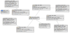
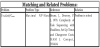
The partner in the first use case produces animal feeds for the local industry. The company has two production lines which work separately and the feed that is produced in one line cannot contaminate the other line. The use case focuses on the main production line, which is used most of the time. The company has 22 products that are produced on this line, and each product is represented by a single operation on the main line. An overview of the process is given in figure 4.

Figure 4: Partner 1 process.

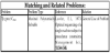
The lines were imported into the tool as shown in figure 5. The classification tool was run on the model and the classification shows hat the process is a single machine problem with a known maximal polynomially solvable solution as shown in figure 6.

Figure 5: Partner 1 Production line representation in tool.

Figure 6: Partner 1 classification result.

6.2 Use case 2

The second example involves a partner whose product is manufactured using 4 machines in a direct line and 3 operators. The machines produce the individual components that are required for the product while the operators assemble the individual parts into the finished component. An overview of part of the process is given in figure 7.

Figure 7: Partner 2 process.

In this scenario, since all the processing is done in sequence, the model is represented as a single machine in the model. This use case indicates that the capacity of the flowline is of 1,200 units per hour, thus indicating that each unit requires 3 seconds to manufacture.

An interesting feature of this use case is the presence of setup times between different jobs. Changing from one job to another requires changing large moulds that are used in the injection moulding process. To replace the mould, calibrate and test the machines, the process takes around 48 hours.

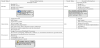
Figure 8 shows the model in the modelling tool whereas figure 9 shows the result of the classification. In this case, the tool reported that the problem is maximal NP-Hard and that the problem is solved (i.e.a problem with the same signature already exists in the database indicating a full match).

Figure 8: Partner 2 Production line representation in tool.

Figure 9: Partner 2 classification result.

5.3 Use case 3

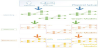
The use case with the third partner involved the manufacturing of a product where subunits can be manufactured in parallel in different work centres. While certain subunits can be done in parallel, there is also an element of precedence, where one task is dependent on another to complete before it can be processed.

The individual work centre will represent a flow line in the model. The sequences and sub-sequences in the model are shown in figure 10, and are defined in the tool through a separate process within the tool.

Figure 10: Partner 3 process for a product with subsequences.

The classification report generated by the tool in this case will contain a section for each in subsequence detected. In fact, for each subsequence in the model, a signature for the sequence is generated and a classification included in the output of the tool. Figure 12 shows a particular result for a subsequence in the model.

Figure 11: Partner 3 - Representation of parallel sequences in tool.

Figure 12: Partner 3 classification result - for a subsequence.

7. Conclusion

The present version of the system is capable of modelling simple production lines with simple single machine, classic parallel machine problems and problems involving routing (such as Flow Shops, Job Shops and Open Shops). Additional problem types are currently being added to the database which includes full referencing to the published works.

A future extension to the project will involve extending the engine to handle models with batch processing, limits on machine processing, and buffers for flow shops.

Competing Interests

The authors declare that they have no competing interests.

Acknowledgments

The project is funded in part by the Malta Council for Science and Technology under the European Research and Development Fund.