


1. Introduction
1.1 Context: ownership identification of reindeer calf
Reindeer herding is the major economic activity of the Sami people, who are the indigenous people of northern Sweden, Norway and Finland. The Sami people lived and worked in reindeer herding groups, which consisted of different families within a designated area and which were formed of working partnerships, where members had individual rights to resources, but helped each other with the management of the herds, or when hunting and fishing. Reindeer husbandry in Norway today is a small industry on a national scale, but is important economically and in employment terms; it is also one of the most important parts of the Sami culture. Reindeer herding in Norway was regulated in 2007 and allowed only those who have the right to a reindeer earmark to undertake reindeer husbandry in the Sami reindeer herding area. This condition applied only to persons who are Sami themselves, whose parents or their grandparents have or had reindeer herding as their primary occupation. A reindeer earmark is a combination of one to many cuts in a reindeer’s ears, which all together tell who the reindeer owner is. There are around 20 different approved cuts in addition to some 30 different combinations of cuts, which have their own names. A committee is in charge of approving earmarks before they are implemented and all reindeer in the Sami reindeer husbandry area shall be marked with the owner’s registered earmark by 31 October the same year as it is born. Reindeer are semi-wild and require large areas for their grazing, they are also often frightened and are forced to flee from natural pastures. Most of the time, they are left to wander freely unaccompanied with their herders [1]. Reindeer herders typically make two migrations with their animals each year. During winter, reindeer are left to breed in the highlands, but just before spring, when food becomes scarcer in the mountains, natural instinct directs the herd to migrate to the low grounds for greener pastures [2]. Reindeer are intercepted by their herders and are taken to the spring pastures before the snow melts and before the mothers start calving. In spring, they move back to the mountainous coastal region where they feed throughout the summer, the calves are soon born and stay with their mothers for protection [3]. In autumn, the herders return to the grazing locations to gather the reindeer from the mountains before the breeding season starts. This is the time when the new calves are branded. Each calf is captured, vaccinated and is given an identification tag or ear mark to distinguish which cow the calf belongs to and to which owner they belong [2]. As meat production became more important since the beginning of the 20th century, reindeer herding became more extensive and Sami reindeer herders started to implement modern technologies, such as snow mobiles and various other mechanical and electronic aids, which became a major feature of modern reindeer herding. Among those technologies, ear identification tags are being used extensively. However, identifying the ownership of new born calves remains a major problem for reindeer herders [1]. Recognizing and matching reindeer calves to the different mothers is traditionally performed in two steps; first, the animals are gathered in a small pen. All female reindeer get individual numbers sprayed on the skin at each side of the animal. Each owner uses one specific color. Unique number plates are hanged to collars around the necks of the calves. Thereafter, the animals are released to larger pens to calm down and are put under surveillance by reindeer owners and herders using binoculars, in order to identify which reindeer calf is following which cow. Thereafter, reindeer owners compare the different observations to guaranty that the correct mother is matched to her calf [4]. The next step is to gather the reindeer herd again in a small pen, capture the calves, remove the number plates and replace them with the approved ear cutting or a tag. This handling procedure is a painstaking process, which demands considerable amount of man power, and long periods of observation of the herd, and is stressful to both herders and animals alike [4]. With the advancement of wireless communications and the wide spread of wireless networks, it has become possible to utilize those technologies for the benefits of reindeer herders and their animals. This paper proposes a technique based on WSN technology for ownership identification of new-born reindeer calves. Various prospective identification technologies such as RFID tag, GPS collars or UHF nodes and gateways are discussed in this work to explore their feasibility for the proposed application [1]. In this concept, it is proposed to equip the reindeer cows and calves with transmitter devices of the selected technology, and monitor the movement of the herd in a confined space, facilitated with a grid of signal receivers, corresponding to the transmitter device attached to the reindeer. A suitable algorithm has to be devised to analyze the gathered data and recognize the pairs of tags which keep close together most of the time, which are reckoned to be the mother reindeer and her calf.
1.2 Overview of WSN-based localization techniques
The problem of self-localization involving low-cost radio devices in wireless sensor networks (WSN) can be viewed as an example of the Internet of Things (IoT). Among the several applications related to this problem, location services may be namely offered by small devices carried by persons in indoor environments. Over the last ten years, several overview papers dealing with the description and classification of localization techniques in this context have been published (see, for instance, [5-7]).
In this work, we focus on the ranging technique relying on received signal strength indicator (RSSI) for indoor scenarios. In [8], the RSSI metric has been related to the Euclidean distance through a lognormal shadowing model (LNSM) describing the signal propagation in free-space. A first approach consists of assuming the LNSM and applying a classical maximum likelihood estimator (MLE) to compute the nodes’ positions. This has been proposed, for instance, in [9], where the parameters of the propagation model are considered equal for all landmarks (i.e., nodes whose positions are known, also called anchor nodes). Following the same approach, the parameters have been considered different for each landmark in in [10]. The experimental results there obtained on real test beds show a mean localization accuracy of 1m.
When dealing with closed and relatively small spaces, RSSI is not accurate enough and the effects of multipath, possible blocking objects and antenna orientation may be also included in the propagation model as outliers (see, for instance, [11,12]). A biased-maximum likelihood estimator (B-MLE) involving a random factor related to the possibly outliers has been studied in [13], this estimator has been experimentally proved to reduce the mean error of the classical MLE. The optimization problem is defined for each single unknown position given several RSSI values from a set of surrounding landmarks.
Our work aims to solve the localization problem of a set of nodes’ positions in a distributed and cooperative way, i.e., both landmarks and neighboring nodes communicate and the data processing and computation is hold by each sensor node without the need of sink nodes (e.g. central station). As the likelihood function of the LNSM is not convex with respect the unknown positions, a basic gradient descent method suffers from the initialization issue. We take inspiration from the two phase methods of [14,15], which consider an initial guess step followed by a cooperative refinement step. In order to improve the accuracy achieved by the B-MLE [13], we use the on-line distributed stochastic approximation (DSA) approach of [16] to minimize the mean square error of the estimated distance derived from the noisy RSSI received data. The iterative DSA algorithm involves a first local update based on stochastic gradient descent (see [16]) given a new RSSI measurement at each sensor node. Then, an asynchronous communication step (see [17]) involves the exchange of information between two randomly selected nodes to reach a consensus on the set of estimated positions. It allows each sensor node to build a local map of itself and its neighbor nodes. Our approach is tested on real indoor scenarios: the two rooms from [18] and a number of selected sensor nodes from the FIT IoT-LAB Rennes platform [19] (platform previously known as SensLAB where the new generation of sensor nodes ARM Cortex M3 with ATMEL radio chipset will be gradually incorporated).
The paper is organized as follows. First, Section II gives an overview of the proposed concept. Section III introduces the notation in use throughout the paper and recalls the lognormal shadowing model (LNSM) for the observed signal. The main equations of the biased lognormal shadowing model (B-LNSM) are introduced in Section IV-A. The initialization phase of the localization algorithm proposed here is presented in Section IV-B, while the refinement phase is detailed in Section V. Section VI describes the test bed of our experimental results, which are subsequently summarized, compared and discussed. Finally, conclusions are provided in Section VII.
2. WSN-Based Reindeer’s Calf Identification Concept
A technique based on wireless sensor networks to identify the ownership of the calves is presented in this work. It is proposed to furnish the new born calves with an electronic identification device, such as RFID tags, GPS collars or UHF nodes, with a system setup facilitated with receivers, gateways and necessary software. The reindeer herd is confined in a restricted space, which is equipped with a grid of signal receivers, corresponding to the transmitter devices attached to the reindeer, and using proper localization algorithms. Movement of transmitter tags is tracked in order to recognize the pairs of tags which keep close together most of the time, which indicate the mother and calf reindeer. Due to the fact that reindeer is a wild animal species, they tend to be more cautious than domestic animals; hence they tend to avoid confined spaces and close objects mounted by humans, which makes the use of passive RFIDs less efficient due to their low range, as the receivers have to be placed at a close proximity to the RFIDs. This demands the application of active RFIDs to both mothers and calves, or the use of other sensor network devices such as GPS collars or UHF nodes and respective gateways. For example, active RFID tags operate at higher frequencies than passive tags because of their on-board power source, commonly 455 MHz, 2:4 GHz, or 5:8 GHz- depending on application’s read range and memory requirements. Readers can communicate with active RFID tags across 20 to 100 meters. In the same way, tags can track the movement of highly mobile objects in wider areas than passive tags [20]. In this procedure, the pen where the animals are to be gathered for tagging is facilitated with a WSN, assuming that the WSN is readily available with a set of low cost sensor nodes such those used in Section VI (WSN430). Central sensor nodes are mounted on posts at the centers of the circles indicated in (Figure 1), which indicate the coverage range of the routers.
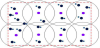
Coverage of the wireless network is configured in such a way to ensure exposure of the whole pen, with minor inevitable pockets of uncovered areas, which have to be kept to a minimum. RFID tags are tracked and location data is logged into a computer program, where data is analyzed to match couples of tags together.
3. Framework
The following framework to solve the localization problem in a distributed manner using WSNs, i.e. local measures and communications through the network of sensor nodes, is based on the previous work proposed in [21].
3.1 Notation
Consider the context of N sensor nodes placed within a two-dimensional
space p × qm2 whose unknown positions are defined by
the set {Zi}∀i which is also represented by every pair of coordinates as
{(x1-y1),...,(xN,yN)}. The euclidean distance between each pair
of nodes i and j is defined as
3.2 Benchmark: log-normal shadowing model (LNSM)
We recall the empirical model used to describe the received signal
strength indicator (RSSI) data as a function of the distances between
the sensor nodes. The log-normal shadowing model (LNSM) is
based on the log-distance path loss model of [8], which describes the
average path loss PL(d) expressed in dB for a distance d as
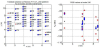
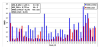
The above equation (1) depends on the propagation parameters P0, η and σ2, which may not be homogeneous in indoor scenarios. A maximum likelihood estimator (MLE) can be used to learn these parameters from the RSSI values collected from a set of landmarks whose positions are known. Since the average values of the RSSI measured at different positions do not always decrease with the distance (see the learning phase in [10]), we let the parameters of the propagation model differ from one landmark to another. As a result, we do not treat all landmarks equally during the statistical estimation (cf. Tables ?? and 1). Moreover, in order to show how, in general, the definition (1) does not match in a real indoor environment, (Figures 2) highlights the presence of a bias probably due to multipaths. For instance, in Figure 2 node 240 collects (27; 7; 21; 203; 26; 533) packets from landmarks whose identifiers (Node_ID) are (157; 163; 176; 214; 236; 244). There is a bias in values coming from landmark 244, even if this is the one closest to node 240. This sensor node is placed at the boundary and immediately close to the wall of the room.
4. Position Estimation: Intialization
4.1 Principle: biased log-normal shadowing model
This section recalls the dynamic method introduced by [13] to
estimate the position of a sensor node from a set of landmarks. The
sensor node seeks to reduce the effect of any potentially aberrant
landmark whose measurements do not improve localization accuracy.
This effect is compensate by introducing a constant bias which
becomes an additional variable to estimate and replaces the lognormal
shadowing model of the measurements associated to this
landmark. Let us denote by RSSIj;L the jth RSSI sample measured by the
sensor node on packets coming from a given landmark L. If we denote
by P0,L,ηL and
where dL is the distance to landmark L that we try to estimate and 1 is the indicator function, which is equal to 1 when the subscript expression is true and 0 otherwise. Abnormal landmarks can be detected from equation (2), and the biased LNSM can be fully characterized. Thus, the biasedmaximum likelihood estimator may be used to compute the sensor node position from RSSI measurements collected from M landmarks. The aberrant landmark can be identified by comparing the global likelihood values when each landmark is considered as outlier.
4.2 Biased-maximum likelihood location estimation method (B-MLE)
Combining all the measured values altogether, we can apply a maximum likelihood estimator on this new model to compute the likelihood expressions in the case where landmark O is considered as abnormal. If we denote by TL the number of samples received from landmark L, the likelihood function is expressed as follows for every landmark L≠O:
and for the outlier (abnormal) landmark, O, it becomes:
The global likelihood function from the data set, reflecting the coherence of the whole system when landmark O is the outlier one is then simply the sum of equations (3) and (4) over the M landmarks:
Thus, the maximum likelihood criterion applied to equation (5) is used to infer the sensor node position and the bias. Using the fact that it can be solved by separating the problem, the B-MLE solution is given by:
Where
5. Position Refinement: Improving The Accuracy
5.1 Principle: distributed stochastic approximation (DSA)
The objective in this phase is described under a global maximum
likelihood estimation of the log-distances between the N sensor nodes
positions. From the LNSM in equation (1), we define the estimated
log-distance
We define the sets of RSSI measurements collected for each sensor
node i as
Where
5.2 On-line gossip-based implementation
Problem (8) is solved by means of the on-line distributed stochastic
approximation algorithm (DSA). At any time t ≥ 0, each sensor node
i updates the sequence of its estimated neighboring nodes’ positions
[Local gradient descent step][16] At iteration t each sensor node
i computes a temporary estimate of its positions’ set from the local
current measurements
Where
[Gossip averaging step] [17] At each iteration time t two uniformly random selected nodes exchange their common estimated positions and average their values. The final updates are set as follows:
Otherwise,
6. Numerical Results: Experiences From WSNS
For the considered testbeds, the procedure is described as follows.
Each of the M landmarks broadcasted 100 frames. Then, the first NL
sensor nodes selected for the learning phase computed the set of the
propagation model parameters
6.1 Testbed description: FIT IoT-LAB platform
The testbeds were chosen at the FIT IoT-LAB’s platform of size 5 ×9m2 involving the positions of 44 sensor nodes and 6 landmarks which are located in a big storage room of size 8 ×11m2 containing different objects. Sensor nodes are placed at the ceil which is 1:9m height from the floor in a grid organization. There was no one in the room most of the time and there was only a wireless access point located in the corridor which is separated by a cinder wall (no electromagnetically isolating). The estimated parameters are summarized in Table 1.

6.2 Comparison and discussion
We have tested the algorithms proposed in Sections IV-B and V-B
whose respective procedures are defined by equations (6) and (9)-
(10). In order to evaluate the performance of such methods and
quantify the achieved accuracy, we define the normalized mean
deviation (NMD) as the average mean deviation (MD) error of the N
estimated positions normalized by the testbed dimensions i.e. p ×qm2.
It can be defined as:
Where
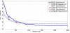
Figure 3 shows the evolution of the mean deviation error MD as a function of the iterative steps during the refinement phase, which involves the communication between two sensor nodes at each step. The earliest improvement (24 steps) has been obtained in Experience 2 of the testbed. However, for this experience the accuracy after the refinement phase has been the worst achieved as the curve of the mean deviation error remains always above. The best accuracy was achieved at Experience 1 for the considered testbed even if the convergence was slower and 89 refinements steps were required to improve the mean deviation error. As reported in Table 2, less than 80 cm was obtained from Experience 1 of the testbed.
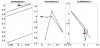

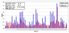
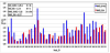
Figure 5 , 6 and 7 show the corresponding normalized NMD values
of each sensor node position
In order to summarized the results for each testbed, Table 2 displays
the average error, both MD in meters and the respective normalized
value as NMD. The numerical results are reported when considering
the two sizes of data sets chosen during the learning phase of the
B-MLE (NL = 10 and NL = 25). In addition, we computed the ratio of
the accuracy improvement as the percentage
7. Conclusion
In this paper, a novel application of WSN based on RFID tags is addressed for ownership identification of new-born reindeer calves, in order to mark the calves with ear marks or identification tags of their relevant owners. The principle of identification is based on matching reindeer calves to their mothers through estimating their locations in the herd, while finding a proximity between a reindeer cow and her calf. In the proposed set-up, active RFID ear tags, which are fitted to the animals, are utilized as nodes. Such tags normally have an accuracy of 3 - 5 meters when determining the location, and when used with central nodes (gateways), it is possible to allow a large number of tags to communicate simultaneously with a single access point without choking the wireless network. The traditional RFID technology would have required a larger number of readers, in order to determine the location of a single tag, with the same precision as the wireless network. For the proposed application, the system needs the implementation of a localization algorithm. Various localization techniques relying on distance measurements in WSNs (related to RSSI magnitude) have been considered and thoroughly discussed in this paper. Several existing techniques has been investigated to estimate locations of target tags considering range measurements, which can be employed in proper computer algorithms to analyze the gathered data-base of animal tracking. Among all possibilities, RSSI is considered here as the most economic and practical choice for the proposed application. Since the accuracy of the estimated positions is not the priority, we proposed a more flexible and cheaper solution thanks to a distributed algorithm. The implemented algorithm is based on local measurements and communications through neighboring nodes. In particular, we considered two phases including an initialization MLE phase and a refinement phase based on a DSA algorithm. The latter enables each sensor node to track its own position and those from its neighbors. This leads the process of matching a reindeer calf to its mother in a robust way. The advocated method suffers from a few limitations pertaining to the number of tags that can be covered using one central node reader and coverage of the pen area, where the reindeer herd is gathered for identification, which could create further problems pertaining to transmission, repeatability and accuracy. The proposed method reduces the amount of effort and time in performing the identification process and paves the way for the implementation of wireless sensor network enabled RFID tags for animal welfare.
Competing Interests
The authors declare that they have no competing interests.