


1. Introduction
In current clinical practice, the 3D size, shape and location of a tumor is often an important diagnostic reference. However, the majority of medical imaging instruments only provide twodimensional (2D) images, although a few expensive instruments can provide three-dimensional (3D) images by stacking the original 2D images, but these 3D images are unprocessed and often cause problems in segregating the target from a mix of complex tissues. Therefore, it is important to have the skills of segmenting the designated object from medical images so it can improve the diagnostic accuracy of doctors, or even become a guide of the surgery. In the previous studies, many two-dimensional (2D) image segmentation techniques have been developed, such as the region growing, zero-crossing [1], region-based segmentation [2], active contour model (ACM) [3], and the level set method (LSM) [4-6]. However, breast MRI tumor segmentation has always been a challenging task because of the low resolution, and the tumor tissue is often mixed with a number of other tissues. Among older segmentation methods, some use the local characteristics; these methods are not stable in the accuracy of segmentation. Some use the gradient as a basis for segmentation; these methods are likely to cause misjudgments on images with vague edges. In addition, some methods are based on intensity; these methods are relatively susceptible to noise interference. Nevertheless, there are also some methods-such as LSM and multi-spectral detection technology [6]-that do give good results for tumor segmentation in breast MRI.
Currently, the segmentation of 3D medical images has become a computer-aided diagnostic technology in dire need of development [7-8]. Since the technologies of 2D image segmentation and contour detection are now relatively mature, so the approach to 3D image segmentation in some parts of the literature is to segment the tumor in each 2D image slice, and then stack these segmented slices to obtain a 3D tumor model [9-11]. Such an approach not only increases the operating cost because of the separate processing of each slice, it also lacks a reference between the upper and lower slices. For this reason, there may be confusion when establishing the 3D model as to the imperfect correspondence between slices, which could greatly reduce the efficiency and accuracy of the 3D segmentation-model reconstruction. In addition, there are some existing 3D image-segmentation techniques and methods that split three orthogonal 2D planes and combine them into a 3D segmentation model [12-14]. Since such an approach does not operate directly on the entire 3D model, it is not considered strictly to be a complete 3D segmentation algorithm.
In order to overcome the problems encountered in the past and segment a more accurate 3D breast tumor model to provide physicians with a diagnostic reference, this paper proposes a new 3D tumor segmentation method, namely, the 3D Modified Active Contour Method (3D-MACM). 3D-MACM not only reduces the computation time but also operates directly on the entire 3D model which conducts the interaction between each pixel and its neighboring points on all three axes (X, Y, and Z). To verify experimentally the feasibility of the proposed method, this paper uses an actual breast MRI case with tumor and several simulated MRI cases for system evaluation. In the course of the experiment, the tumor is first segmented and a 3D model of the tumor is rendered from the segmentation results using the Marching- Cubes-Isosurface (MCIS) method. A quantitative evaluation is then conducted according to the standard model (delineated by physicians for actual breast MRI case), and the effectiveness of the algorithm is verified using this quantitative data. Finally, the accuracies and false alarm rates of traditional ACM and 2D/3D LSM are compared to demonstrate the advantages of 3D-MACM.
This paper is organized as follows. Section 2 will introduce 2D-ACM and the new approach 3D-MACM proposed in this paper. The experimental arrangements and results are described in Section 3. Finally, conclusions are presented in Section 4.
2. Methods
2.1 Two-dimensional Active Contour Method (2D-ACM)
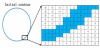
An initial closed curve (initial contour) must first be defined, followed by the definition of a circular shape; and the initial contour explains each pixel to form the image height distribution map which outside the contour gradually increases and inside the contour gradually decreases, as shown in Figure 1.
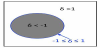
This divides the entire image space into three parts: one in which pixels with -1 ≤ δ ≤ 1 are on the contour line, a second one in which pixels with -1 ≤ δ are inside the contour, and a third one in which pixels with δ ≤ 1 are outside the contour, as shown in Figure 2. The values of are updated constantly according to the update function. In the meantime, the contour also changes and gradually approaches the object. Finally, when convergence is achieved, pixels with -1 ≤ δ ≤ 1 form the final contour of the target object.
2.2 Three-dimensional Modified Active Contour Method (3D-MACM)
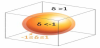
The development of 3D-MACM is an evolution based on twodimensional active contour method (2D-ACM). When the latter is applied in 3D medical image segmentation, only the effect between pixels on the same slice can be taken into consideration during the whole process. This is because each 2D slice has to be processed separately, and those processed 2D matrices are then used to form the 3D matrix to construct a 3D model; pixels on different slices cannot be linked. Unlike 2D-ACM, the 3D-MACM developed in this paper adds a third dimension to the algorithm, i.e., the Z-axis. This enables pixels on different slices to be associated with each other. The process is first to stack the 2D MR image slices to obtain a 3D matrix, and to perform calculations in the overall 3D space; and then the effectiveness will be predictably much better than that of 2D segmentation techniques. In this paper, the proposed 3D-MACM first expands a 2D contour line to a 3D contour surface on the basis of the initial contour definition, where pixels with -1 ≤ δ ≤ 1 are on the contour surface, pixels with -1 ≤ δ are inside the 3D contour surface, and pixels with δ ≤ 1 are outside the 3D contour surface, as shown in Figure 3.
Since the 3D-MACM update equation must take the Z-axis into consideration, this paper redefines the update equation, as shown in Eq. (1):
where σ and μ represent the weighting factor of the image and
μ0 is grayscale values of pixel at position (x,y,z); the terms c1 and c2
represent the averages of the internal and external grayscale values
of the contour surface, respectively. is an adjustable constant for
controlling the sharpness of the pulse. The term
In 3D-MACM, the consideration of the gradient on the Z-axis of the contour surface is needed, so this paper provides a new definition, as shown in Equation (2). xy, yz, and xz represent the gradient quantization values on the X-, Y- and Z-axes of the image, respectively. In addition, redefining the initial contour will be operated in which pixels with -1 ≤ δ ≤ 1 after using the junction of positive and negative.
2.3 Three-dimensional Surface Rendering (3DSR)
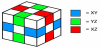
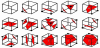
In the results obtained via the 3D-MACM operation, all the pixels with -1 ≤ δ ≤ 1 form the 3D contour matrix, and the process of converting this matrix to a 3D surface is referred to as threedimensional surface rendering (3DSR). 3DSR approach broadly includes two categories: the light projection method [15,16] and the iso-surface approximation method [17,18]. Some typical techniques contain Volume Rendering (VR) [19,20], Contour-Tracing Iso- Surface (CTIS) [21], Marching-Cube Iso-Surface (MCIS) [18], and etc. In this paper, we use the Marching-Cube Iso-Surface (MCIS) method to construct the breast tumor 3D model because of his excellent performance. The MCIS is a way to construct an iso-surface on an object surface is to treat the small cubes in the 3D space as the basic units, and to find the respective iso-surface of each one. When a cube has eight vertices and each vertex has two states (marked and unmarked), there are 28 = 256 possible distributions of iso-surfaces. However, taking into account the rotational symmetry of a cube, there are only 15 different cases, as shown in Figure 5.
The corresponding iso-surface can then be generated quickly within the small cubes according to a lookup table. The MCIS calculation process can be described in more detail as follows.
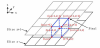
- Read in adjacent two planes (X-Y planes) of the matrix at a time, forming a layer and a cube which constituted by four corresponding points from the upper and lower planes, as shown in Figure 6.
- Process all the cubes in a layer sequentially (extract the isosurface of each cube), and then process each layer from bottom to top in the object.
- For each cube, the grayscale values of its eight vertices can be obtained directly from the 2D planes, and the threshold of the isosurface to extract is known (set by the user). If the grayscale value of a vertex is greater than the set value, it becomes a marked vertex (black), while a vertex with a grayscale value less than the set value remains unmarked.
3. Experimental Data and Results
3.1 Establishment of experimental data and evaluation criteria
The research adopted two kinds of images for the 3D tumorsegmentation experiment and performance evaluation, including simulated MR images and actual breast MR images. There are two reasons to use simulated MR images in the primary experiment.
- The characteristics of simulated MR images can be accurately grasped.
- Simulated MR images can provide more objective results of segmentation.
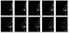
For the actual breast MRI case, the imaging sources are from Tri- Service General Hospital, Taipei, Taiwan. The resolution of each image is 512 × 512. The chosen case has 98 image slices with a slice spacing of 2mm, and the scope of slices contain the tumor site. Figure 7 shows partial slices of the actual breast MRI case with breast tumors.
In order to perform systematic quantitative evaluation for the actual MRI case, the evaluation criteria first had to be established. For slices with the tumor image in actual MRI case, three experts delineated the tumor outline. The intersection area was taken as the standard contour, and a standard 3D tumor contour was further established in combination with the standard contour in each slice. In the subsequent experiments, systematic performance evaluation and quantitative analysis was conducted based on this standard 3D tumor contour.
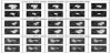
Simulated MR images are simulated from actual MRIs, and the gray-level distribution is obtained from the average sampling points of the tissues in actual breast MR images. In order to make the simulated image closer to the actual MRI, a variety of simulated images separately added the noise with density of 30%, 40%, and 50% as well as blurred by using 3 x 3, 5 x 5, and 7 x 7 mask. Partial slices of a simulated MRI case with different noise densities and blurring are shown in Figure 8.
3.2 Systematic evaluation methods
To evaluate the performance of 3D-MACM, this study conducts the correct classification rate (CCR), specificity (SP), and false alarm rate (FAR) which are the commonly used evaluation indices in a variety of medical aided systems. Meanwhile, the performances also compare with different existing algorithms. Each evaluation index is calculated as follows:
where N represents the total number of pixels in the threedimensional region of interest (3D-ROI), and Nn represents the total number of pixels outside the standard 3D tumor contour in the 3D-ROI. The acronym TPN stands for True Positive Number, which represents the number of pixels inside the standard 3D tumor contour and also detected as the pixels inside standard 3D tumor contour. The acronym FPN stands for False Positive Number, which represents the number of pixels outside the standard 3D tumor contour but detected as the pixels inside standard 3D tumor contour. The acronym TNN stands for True Negative Number, which represents the pixels outside the standard tumor contour and also detected as the pixels outside standard 3D tumor contour. The acronym FNN stands for False Negative Number, which represents the pixels inside the standard tumor contour but detected as the pixels outside standard 3D tumor contour. The closer CCR and SP are to 100%, the more accurate the detection result of the algorithm will be. Finally, FAR is a system error indicator, whose percentage should be as low as possible.
3.3 Establishment and comparison of 3D tumor-segmentation models
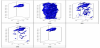
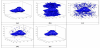
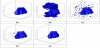
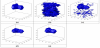
In this section, we use traditional ACM, LSM, 3D-LSM and the 3D-MACM which proposed in this paper to perform 3D tumor segmentation on the experimental cases. The resulting 3D tumor contour matrix is converted to a 3D surface (3D tumor-segmentation model) via the 3DSR process of MCIS in order to observe and compare the results. The actual MRI case has a tissue type of relatively more glandular, and both the breast and tumor sizes are relatively small. The segmentation results of this case are shown in Figure 9. In addition, the segmentation results of simulated tumor cases are shown in Figure 10- 12. As Figure 9 and Figure 10-12 have shown, figure (a) is the standard 3D tumor model; figures (b–e) are the 3D tumor-segmentation models obtained by ACM, LSM, 3D-LSM and 3D-MACM, respectively. The following conclusions can be drawn from these 3D tumor-segmentation results. The results in Figures 9 and Figure 10- 12 show that the 3D tumor-segmentation model generated by the 3D-MACM proposed in this paper is the one that is most consistent with the standard 3D tumor model. When 2D segmentation techniques evolve into 3D techniques, the application of 3D segmentation gives good performance because the upper and lower slices are connected.
3.4 Quantitative Evaluation and Comparison
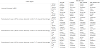
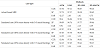
This section performs quantitative analysis based on the standard 3D tumor contours (Figures 9(a) and 10(a)-12(a)) for the 3D tumorsegmentation results of each case, and compares the quantitative results of 3D-MACM with those of ACM, LSM and 3D-LSM. Table 1 shows the TPN, FPN, TNN, FNN, Np, Nn and N numbers of the different algorithms in each case, where Np is the total number of pixels inside the standard tumor contour and hence represents the actual size of the tumor. It can be seen from the data in Table 1 that in all cases the total amount of correctly segmented pixels with 3D-MACM is the highest, and that its number of wrongly segmented pixels is the lowest. It explains that TPN and TNN represent the numbers of pixels segmented correctly, while FPN and FNN are the numbers of pixels wrongly segmented. The three kinds of evaluation indices used commonly in medical aided systems (CCR, SP and FAR) can be deduced from the data in Table 1 and the calculations of Eq. (3–5), as shown in Table 2. From that table, it can be seen that LSM has a better performance in 3D tumor segmentation than that of ACM. Evolving from LSM to 3D (3D-LSM), can improve CCR and SP effectively, as well as reducing the false alarm rate (FAR). However, 3D-MACM gives the highest CCR and SP, and the lowest FAR. This quantified performance is consistent with the observation results of the 3D tumor-segmentation models in the previous section. This proves again that the application of 3D-MACM in 3D tumor segmentation can eliminate background noise effectively, so that the segmented contour is closer to the actual tumor margin.
4. Conclusions
3D medical image segmentation is used to segment the target (a lesion or an organ) in 3D medical images. Through this process, 3D target information is obtained; hence, this technology is an important aided tool for medical diagnosis. This paper presents an innovative 3D medical image-segmentation method called the 3D Modified Active Contour Method (3D-MACM), which can segment the target lesions precisely from 3D medical images. Most of the 3D segmentation algorithms will be affected largely by errors and/or noise. Although many 2D segmentation methods have proved successful in the past, the 3D image segmentation obtained by segmenting 2D slices individually and then stacking them has not been satisfactory due to the lack of connectivity between the upper and lower slices. Therefore, 3D-MACM combines the information of the upper and lower segments, and then recalculates with the simple initial contour which not only brings the segmented contour closer to the actual outline of the tumor margin, but also accelerates convergence and eliminates background noise.
In order to validate our proposed method, this study used actual breast MRI and simulated cases with different noise and blurred masks for evaluation. In the experiment, 3D models of the tumors were constructed using the segmentation results through MCIS in order to facilitate visual observation and comparison. This was followed by a quantitative evaluation to verify the effectiveness of the algorithm with quantitative data. Finally, the accuracies and error rates of traditional ACM, and 2D/3D LSM were compared. The experimental results show that the method developed in this paper (3D-MACM) not only has more accurate contour and less noise than the traditional methods, but it also has the highest accuracy and lowest false alarm rate in comparison with the standard model.
Competing Interests
The authors declare that they have no competing interests.