Profile
International Journal of Computer & Software Engineering Volume 2 (2017), Article ID 2:IJCSE-112, 7 pages
https://doi.org/10.15344/2456-4451/2017/112
Review Article
An SOM-Like Approach to Inverse Kinematics Modeling

Mu-Chun Su* and Chung-Cheng Hsueh

Department of Computes Science and Information Engineering, National Central University, Taiwan
Prof. Mu-Chun Su, Department of Computes Science and Information Engineering, National Central University, Taiwan; E-mail: muchun@csie.ncu.edu.tw
14 January 2017; 16 February 2017; 18 February 2017
Su MC, Hsueh CC (2017) An SOM-Like Approach to Inverse Kinematics Modeling. Int J Comput Softw Eng 2: 112. doi: https://doi.org/10.15344/2456-4451/2017/112
This paper was partly supported by supported by Ministry of Science and Technology, Taiwan, R.O.C, under 106-2221-E-008-092, 105-2218-E-008-014, and 104-2221-E-008-074-MY2.

Abstract

Robot kinematics modeling has been one of the main research issues in robotics research. For realtime control of robotic manipulators with high degree of freedom, a computationally efficient solution to the inverse kinematics modeling is required. In this paper, an SOM-Like inverse kinematics modeling methodis proposed. The principal idea behind the proposed modeling method is the use of a first-order Taylor series expansion to build the inverse kinematics model from a set of training data. The work space of a robot arm is discretized into a cubic lattice consisting of Nx×Ny×Nz sampling points. Each sampling point corresponds to a reciprocal zone and is assigned to one neural node, storing four different data items(e.g., coordinates position vector, template position vector,the joint angle vector, and the Jacobian matrix) about the first-order Taylor series expansionof the inverse kinematics function at that sampling point. The proposed inverse kinematics modeling method was tested on a 3-D printed robot arm with 5 degrees of freedom (DOF). The performance of the proposed method was tested on two simulated examples. The average approximation error could be decreased to 0.283 mm in the workspace, 200.0 mm×200.0 mm×72.0 mm and 0.25 mm in the workspace, 200.0 mm×200.0 mm.


1. Introduction

Robot kinematics modeling has been one of the main research issues in robotics research. It can be divided into forward kinematics and inverse kinematics. Forward kinematics refers to the calculation of the position and orientation of an end effector in terms of the joint angles, x =f( θ ) where x = ( x 1 , x 2 , x 3 ) T represents the Cartesian position of the end effector and θ =( θ 1 , θ 2 ,..., θ n )t represents the joint angles where we assume there are n joints in the joint configuration. Inverse kinematics refers to find the transformation θ = f 1 ( x ) from the position of the end effector in the external Cartesian position space to the joint angles in the internal joint space. While there is always a straightforward solution to forward kinematics, the solution to inverse kinematics is usually more difficult, complex, and computationally expensive. For real-time control of robotic manipulators with high degree of freedom, a computationally efficient solution to the inverse kinematics modeling is one of the main requirements.

Approaches to the inverse kinematics problem can be roughly categorized into four classes: the analytical approach (e.g., [1-5]), the numerical approach (e.g., [6-11]), the computational intelligence-based approach (e.g., [12-20]), and the lookup tablebased approach (e.g., [21-23]). While the analytical approach solves the joint variables analytically according to given configuration data to provide closed form solutions, the numerical method provides a numerical solution (e.g., the use of the Jacobian matrix of the forward kinematics function, x =f( θ ) to approximate the optimal joint angles [24]. Real-time applications usually prefer closed form solutions than numerical solutions because the latter one either requires heavy computations or fails to converge when a singularity exists. The computational intelligence-based approach provides an alternative solution to the inverse kinematics problem [12-20]. Many co1mputational intelligence-based methods were based on the use of the self-organizing feature map (SOM) [12-14,16-20]. Recently, the lookup table-based approach has been introduced to solve the inverse kinematics problem due to its simplicity [21-23]. Basically, the lookup table-based approach consists of two phases: the phase of the off-line construction of the lookup table and the on-line interpolation phase. The lookup table-based approach may encounter the following problems. First of all, the amount of memory required for constructing an effective table may increase as the number of joints and the resolution of the table increase. In addition, a further approximation procedure may be adopted to search for a better solution once an initial table entry has been located. Without any doubt, each one of the aforementioned four approaches has its advantages and limitations.

The goal of this paper is to endow a 3-D printed humanoid robot arm with the ability of positioning its fingertip to a target position in real time. To achieve this goal, the robot system has to seek a high efficiency solution to inverse kinematics modeling. In this paper we propose an SOM-like approach to solving the inverse kinematics problem. The proposed approach integrates the SOMbased approach and the lookup table-based approach.Our approach is the use of a Taylor series expansion to build the transformation θ = f 1 ( x ) from the position of the end effector in the external Cartesian position space to the joint angles in the internal joint space from a set of training data. The principal idea behind the proposed modeling method is to discretize the work space of a robot arm into a cubic lattice consisting of Nx×Ny×Nz sampling points. Each sampling point corresponds to a reciprocal zone and is assigned to one neural node.Each neural node storesfour weight vectors or data items: the coordinates position weight vector w j c the template position weight vector w j t the joint angle weight vector w j θ and the Jacobian matrix W j J . All these four data terms can be quickly learned by the proposed modeling method from a collected training data set. The training data set can be constructed by either the uniformly discretization scheme or the real-life data generation scheme. The computations of the joint angles corresponding to a target position in the work space involve the following two steps. First of all, we search the reciprocal zone which is closest to the target position. Secondly, the joint angles are approximated by he first-order Taylor series expansion of the transformation θ = f 1 ( x ) via the target position vector x target , the joint angle vector w j θ , and the Jacobian matrix W j J within the reciprocal zone.

The performance of the proposed SOM-like inverse kinematics modeling method was tested on a 3-D printed robot arm with 5 degrees of freedom (DOF). Two simulated examples were designed to test whether the robot arm could successfully position its fingertip to target positions in the work space.

This paper is organized as follows. Following this introduction is a brief review of the Taylor series expansion and the SOM algorithm. Section III explains the detailed descriptions of the proposed SOMlike inverse kinematics modeling method. Simulation results are given in Section IV. The final section contains the discussions and conclusions.

2. Brief Review of the Taylor Series Expansion and the SOM Algorithm

2.1 The Taylor Series Expansion

In mathematics, a vector-valued function can be approximatedvia the first-order Taylor expansion as follows:

F( x )F( p )+J( p )( x p )

where x is a data point, p is a template point, F( x ): n m is a vector-valued function, and J( p ) is the Jacobian matrix at the template point p . The Jacobian matrix J( p ) is the matrix of the all first order partial derivatives of the vector-valued function F( x ) as follows:

J( p )=[ F 1 x 1 F 1 x n F m x 1 F m x n ]

An immediate problem needed to be solved is the estimation of the Jacobian matrix at the point, p . There are two methods to estimate the Jacobian matrix from the N+1 data pairs. One popular method is the use of the Moore-Penrose generalized Inverse operator. Assume we have N+1 data pairs, ( x 1 ,F( x 1 ) ),...,( x N ,F( x N ) ), ( p ,F( p ) ) . Let us rewrite Eq. (1) as follows:

ΔF=J( p )Δp

where

Δp=[ x 1 p x n p ],ΔF=[ F( x 1 )F( p ) F( x n )F( p ) ], and J( p )= [ J 11 J 1n J m1 J mn ] m×n

Since we have N+1 data pairs, ( x 1 ,F( x 1 ) ),...,( x N ,F( x N ) ),( p ,F( p ) ), Equation (3) can be expanded to be as follows:

[ Δ F 1 1 Δ F 1 N Δ F m 1 Δ F m N ] m×N = [ J 11 J 1n J m1 J mn ] m×n [ Δ p 1 1 Δ p 1 N Δ p n 1 Δ p n N ] n×N

Δ F m×N =J ( p ) m×n Δ p n×N

The solution of the matrix J m×n is computed as follows:

J (p) m×n =Δ F m×N ( ( ( Δ p n×N ) T ) ) T =Δ F m×N ( Δ p n×N ) T ( ( Δ p n×N ( Δ p n×N ) T ) 1 ) T

where ( ( Δ p n×N ) T ) is the Moore-Penrose generalized inverse of the matrix ( Δ p n×N ) T .

2.2 The SOM

The training algorithm proposed by Kohonen for forming a selforganizing feature map (SOM) is summarized as follows [25,26]:

Step 1. Initialization: Consider the network on a rectangular grid with M rows and N columns. Each neuron in the neural network is associated with an n-dimensional weight vector w , Randomly choose values for the initial weight vectors w j (0)

Step 2. Winner Finding: Present an input pattern x (k) to the network and search for the winning neuron. The winning neuron j * at time k is found by using the minimum-distance Euclidean criterion:

j * = Arg min 1jM×N || x (k) w j (k)||

where x ( k )= [ x 1 ( k ), x 2 ( k ),, x n ( k ) ] T represents the kth input pattern and indicates the Euclidean norm.

Step 3. Weight Updating: Adjust the weights of the winner and its neighbors using the following updating rule:

w j ( k+1 )= w j ( k )+η( k ) Λ j * ,j ( k )[ x ( k ) w j ( k ) ]for1jM×N

where η(k) is a positive constant and Λ j * ,j (k) is the topological neighborhood function of the winner neuron j * at time k.

Step 4. Iterating: Go to step 2 until some pre-specified termination criterion is satisfied.

3. The Proposed SOM-Like Approach to Inverse Kinematics Modeling

The goal of the proposed SOM-like approach to inverse kinematics modeling is to derive an corresponding joint angles, θ from any fingertip position, x . It involves two phases: (1) the off-line training phase and (2) the real-time manipulating phase. While the off-line training phase is to derive the inverse kinematics model for each sampling point over the discretized work space of the robot arm from a collected training data set, the real-time manipulating phase is to compute the corresponding angles for a particular fingertip position based on the trained inverse kinematics model in real-time.

3.1 The off-line training phase

The proposed off-line training phase integrates the merits of the SOM-based approach and the lookup table-based approach.It fully utilizes the topology-preserving property of the SOM algorithm to generalize the modeling capability from collected data to unknown data space. In addition, similar to the table-based approach, it is able to calculate the necessary information to derive the inverse kinematics with no need of a complicated learning procedure. The principal idea behind the proposed modeling method is to discretize the workspace of a robot arm into a cubic lattice consisting of Nx×Ny×Nz sampling points. Each sampling point corresponds to a non-overlapping reciprocal zone in the workspace. For each sampling point, we will stores four weight vectors or data terms (i.e. w ( k,l,m ) c , w ( k,l,m ) t , w ( k,l,m ) θ  and  W ( k,l,m ) J in order to quickly derive corresponding joint angles θ for any fingertip position x located inside the corresponding reciprocal zone of the sampling point via the first-order` Taylor expansion. All these four data terms can be quickly learned by the proposed off-line training phase.

The off-linetraining phase is describedas follows:

Step 1: Workspace Specification- First of all, we need to specify where the workspace of the robot arm is. Assume that the workspace of the robot arm is located in the region defined by [mx,Mx ]×[my,My]×[mz,Mz] where the parameters, mx,Mx, my,My,mz, and Mz are the lower bounds and upper bounds for the workspace with respective to the axes, X, Y, and Z, respectively.

Step 2: Lattice Determination- Discretize the work space into an equidistant cubic lattice consisting of Nx×Ny×Nz template points. The more template points the workspace has, the smaller the approximation error the training phase will achieve. Accordingly, we set the SOM network structure to be a 3-dimensional lattice structure with the network size, Nx×Ny×Nz. Each neural node isthenrespectively assigned to its correspondingtemplate point. Therefore, the reciprocal zone of each neural nodeis M x m x ( N x 1) × M y m y ( N y 1) × M z m z ( N z 1) . Each neural node then needs to store the its corresponding fourweight vectors: the coordinates vector of the sampling point W (k,l,m) c , the template position vector w ( k,l,m ) t the joint angle vector w ( k,l,m ) θ , and the Jacobian matrix W ( k,l,m ) J . These four weight vectors will be computed in the following steps from a set of training data.

Step 3: Collecting training data- Assume the forward kinematics model of the robot arm has been developed via some kind of forward kinematics modeling method. Based on the generated forward kinematics model, we can easily derive the position of the fingertip of the robot arm from a given combination of joint angles. The training data can be constructed by either the uniformly discretization scheme or the real-life data generation scheme. If we have generated the forward kinematics model then we suggest to use the uniformly discretization scheme. Let RAi and Δθi represent the physical range limit and the sampling step for the ith joint, respectively. Therefore, we will collect N s =( R A 1 Δ θ 1 +1 )×( R A 2 Δ θ 2 +1 )××( R A N act Δ θ N act +1 ) training data, ( θ 1 , x 1 ),( θ 2 , x 2 ),...,( θ N s , x N s ), where Nact represent the number of joint angles. The more training data we collect, the higher the performance of our method will achieve. The prices paid for the high performance are: (1) the need of larger memory for storing the corresponding four weight vectors and (2) the more training time.

Step 4: Training of the SOM network- It involves the following four sub-steps.

(4.1) Initialization: For each neural node, its corresponding fourweight vectors are initialized as follows:

w ( k,l,m ) c ( m x + M x m x ( N x 1) ×k, m y + M y m y ( N y 1) ×l, m z + M z m z ( N z 1) ×m ) T

w ( k,l,m ) t ( m x + M x m x ( N x 1) ×k, m y + M y m y ( N y 1) ×l, m z + M z m z ( N z 1) ×m ) T

w ( k,l,m ) θ ( 0,,0 ) T

W ( k,l,m ) J ( 0 0 0 0 )

(4.2) Winner Finding: Present an input pattern x i to the network and search for the winning neuron. The winning neuron ( k * , l * , m * ) corresponding to the input pattern x i is found by using the minimumdistance Euclidean criterion:

( k * , l * , m * )=Arg min 0k N x 1,0l N y, 1,0m N z 1,0k N x 1,0l N y, 1,0m N z 1 x i w ( k,l,m ) c

(4.3) Weight Updating: Adjust the weights of the winning neuron using the following updating rule:

w ( k * , l * , m * ) t x i

w ( k * , l * , m * ) θ θ i

A flag is attached to each neural node to indicate whether the node has already won one competition. If the node has won for at least one competition then the value of its flag will be set to be one; otherwise, zero. After all Ns training data have been presented to the SOM network, the neural nodes with non-zero flag value are regarded as “template nodes”. On the contrary, neural nodes with a zero flag value are claimed to be “novice nodes”. All novice nodes have to enter the next sub-step to update their weight vectors. One thing should be pointed out is that several neural nodes may have won the competitions for more than one time. If this case happens then the training data with the smallest distance to the coordinates position vector, w ( k,l,m ) c , is adopted to update the particular node’s template position vector via (15).

(4.4) Updating the empty nodes’ weights: In this sub-step, we fully utilize the topology-preserving property of the SOM. We assume that neural nodes have similar responses as their neighboring nodes. Based on this assumption, the weight vectors of a novice node can be computed from its neighboring nodes. For each novice node (k, l, m), we will find how many neighbors of the novice node are already template nodes. We only consider its 3×3×3 neighboring nodes. The novice nodes are sorted in a decreasing order according to the numbers of their neighboring nodes which are template nodes. According to the sorted order, the joint angle vector w ( k,l,m ) θ of a novice node is updated as follows:

w ( k,l,m ) θ = ( i,j,h )N S ( k,l,m ) 1 w ( k,l,m ) c w ( i,j,h ) c ( i,j,h )N S ( k,l,m ) 1 w ( k,l,m ) c w ( i,j,h ) c w ( i,j,h ) θ

where NS(k,l,m) represents the set of template nodes within the 3×3×3 region. After the updating change, a novice node then becomes a template node. This process is repeated until all novice nodes are updated and become template nodes.

Step 5: Computationof Jacobian matrix- According to Equation (1), if the template point p is very close to the data point x then the joint angles θ corresponding to a particular location x can be linearly approximated as follows:

θ( x )θ( p )+J( p )( x p )

where p is a template point with the Jacobian matrix J( p ) . An immediate problem is how to compute the Jacobian matrix for each template point. After Step 4, the neural node located at the sampling point w ( k,l,m ) c has been assigned a template position weight vector, w ( k,l,m ) t , and a joint angle weight vector, w ( k,l,m ) θ . Assume each node has Nnb neighboring nodes. For example, nodes located at the eight corners have only 3 neighboring node but most of the nodes inside the lattice have 26 neighboring nodes. Then we can construct a set of Nnb data pairs for the neural node located at w ( k,l,m ) c to estimate the corresponding Jacobian matrix via (7). To be concise and clear, we denote the Nnb data pairs for h = 1,…,Nnb as follows:

( Δ θ h ,Δ x h )=( w ( k±1,l±1,m±1 ) θ w ( k,l,m ) θ , w ( k±1,l±1,m±1 ) t w ( k,l,m ) t )

These Nnb data pairs should meet the following conditions:

{ Δ θ 1 J N act ×3 Δ x 1 ( Δ θ 1 1 ,,Δ θ N act 1 ) T [ J 11 J 13 J N act 1 J N act 3 ] ( Δ x 1 1 ,,Δ x 3 1 ) T                                                              ... Δ θ N nb J N act ×3 Δ x N nb ( Δ θ 1 N nb ,,Δ θ N act N nb ) T [ J 11 J 13 J N act 1 J N act 3 ] ( Δ x 1 N nb ,,Δ x 3 N nb ) T

where the Jacobian matrix J is a Nact×3 matrix since there are Nact joints and the workspace is a 3-dimensional space. Via (7) the Jacobian matrix can be computed as follows:

J N act ×3 =Δ Φ N act × N nb ( Δ X 3× N nb ) T ( ( Δ X 3× N nb ( Δ X 3× N nb ) T ) 1 ) T

where

Δ Φ N act × N nb =[ Δ θ 1 1 Δ θ 1 N nb Δ θ N act 1 Δ θ N act N nb ]

Δ X 3× N nb =[ Δ x 1 1 Δ x 1 N nb Δ x 3 1 Δ x 3 N nb ]

3.2 The real-time manipulating phase

After the off-line training procedure, an inverse kinematics model has been approximated via a trained SOM network with Nx×Ny×Nz lattice structure. Each neural node stores the necessary information (e.g., the template position weight vector w ( k,l,m ) t the joint angle weight vector w ( k,l,m ) θ , and the Jacobian matrix weight vector W ( k,l,m ) J within the reciprocal zone) for the inference of the first-order Taylor expansion. The trained inverse kinematics model can be used to predict a set of appropriate joint angles θ target given a special targeted position vector, x target .

4. Results and Discussion

Step 1: Initialization: Set the iteration parameter k=0 and set the initial real position vector x ( 0 ) to be the targeted position vector, x target (i.e., x ( 0 )= x target )

Step 2: Winner finding: Present the present positionx x ( k ) to the network and search for the winning neuron. The winning neuron ( k * , l * , m * ) at time k is found by using the minimum-distance Euclidean criterion:

( k * , l * , m * )=Arg min 0k N x 1,0l N y, 1,0m N z 1,0k N x 1,0l N y, 1,0m N z 1 w ( k,l,m ) c x ( k )

We search the sampling point of which reciprocal zone is the closest to the present real position vector x ( k ) . If k> 0, then x ( k )= x real ( k ) which will be calculated at the next step.

Step 3: Calculating the joint angles: The joint angles are approximated by he first-order Taylor series expansion via the joint angle vector w ( k * , l * , m * ) θ , and the Jacobian matrix w ( k * , l * , m * ) J .

θ( k+1 )=θ( k )+Δθ( k )θ( k )+ w ( k * , l * , m * ) J ( x target x real ( k ) )

where x real ( 0 )= w ( k * , l * , m * ) t and θ ( 0 )= w ( k * , l * , m * ) θ .

Step 4: Actuating the joint angles: Let the robot arm move to the new real position, x real ( k+1 ) , according to the joint angles, θ(k+1), computed by the previous step.

Step 5: Termination criteria: If the new real position is close enough to the target position (e.g., the approximation error between the target position and the final real position x real ( k+1 ) x target ϵ where ϵis a pre-specified threshold) then we terminate the procedure; otherwise, we set k = k + 1 and go to step 2 until some pre-specified iteration number is reached.

5. Simulation Results

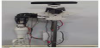
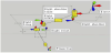
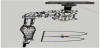
To test the performance of the proposed SOM-Like inverse kinematics modeling method, humanoid robots arm with 5 degrees of freedom was our test platform. The design of the robot arm was from the InMoov project [27]. The InMoov was the first open source 3D printed life-size robot. Based on the open source and a 3D printer, we implemented a humanoid robot arm with 5 degrees of freedom as shown in Figure 1. The Denavit-Hartenberg (DH) method is the most common method to construct a forward kinematics for a robot platform based on four parameters (e.g., the link length, link twist, link offset or distance, and joint angle) [28]. A coordinate frame is then attached to each joint to determine the DH parameters. Figure 2 shows the coordinate frame assignment for the robot arm.

figure 1
Figure 1: The humanoid robot arm with 5 degrees of freedom used as the test platform.
figure 2
Figure 2: The coordinate frame assignment for the robot arm.

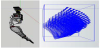
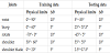
Based on the forward kinematics, 20,800 training data points and 9,072 testing data points were generated, respectively. Figure 3 shows the workspace of these data points. The physical boundaries of these data points and the way for generating the data points are tabulated in Table 1. We then used five different network sizes to discuss whether the network size would influence the approximation performance. Table 2 tabulates the average approximation error, the maximum approximation error, and the computational time. The simulation was done on a PC with 4.0 GB memory, Intel Core i7-2600 CPU @ 3.40 GHz, and the operating system Windows 7. Two observations can be concluded. First of all, the larger the network size is the smaller the average approximation error is reached. Secondly, the larger the network size is the longer the computational time is required. We then took a tradeoff between the approximation error and the computational efficiency to choose an appropriate network size for the following two simulated examples.

figure 3
Figure 3: The workspace of the training data and the testing data.
table 1
Table 1: The physical boundaries of the robot arm.
table 2
Table 2: The approximation performance of the proposed SOM-Like inverse kinematics modeling method with five different network sizes.

After the inverse kinematics model of the robot arm has been constructed, two simulated examples were designed to further test the performance of the proposed SOM-Like inverse kinematics modeling method.

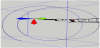
5.1 Example one: Tracking a Circular Helix

The first simulation was designed to track the circular helix defined as:

{ x=157.3+100.0coscosθmm y=387.4+100.0sinsinθmm z=567.7+0.1×θmm

The circular helix was sampled for every Δθ=1° and there were total 720 sampling points. Figure 4 shows the circular helix tracked in the workspace, 200.0 mm×200.0 mm×72.0 mm, with an average error 5.73 mm if the maximum iteration number is only 1. To further decrease the approximation error, the termination criterion parameter ϵ was set to be 0.5 mm so that the real-time manipulating phase took about 0.0306 milliseconds to repeat the iterative procedure for 200 iterations. Finally, the average approximation error decreased to be 0.283 mm.

figure 4
Figure 4: The circular helix tracked by a 10×10×10 SOM model.

5.2 Example two: Writing a letter “B”

The second simulation was designed to write a letter “B” as follows:

Line 1: x=207.7mm,z=638.8mm,493.3mmy293.3mm

Ellipse 1: { x=207.7+200.0coscosθmm y=343.3+50.0sinsinθmm z=638.8mm     90θ90

Ellipse 2: { x=207.7+200.0coscosθmm y=443.3+50.0sinsinθmm z=638.8mm     90θ90

The ellipses were sampled for every Δθ=1° and there were total 360 sampling points. The line was sampled for every 1 mm and there were 200 samples. Figure 5 shows the letter “B” tracked in the workspace, 200.0 mm×200.0 mm, with an average error 6.58 mm if the maximum iteration number is only 1. To further decrease the approximation error, the termination criterion parameter ϵ was set to be 0.5 mm so that the real-time manipulating phase took about 0.0175milliseconds to repeat the iterative procedure. Finally, the average approximation error decreased to be 0.247 mm.

figure 5
Figure 5: The letter “B” tracked by a 10×10×10 SOM model.

6. Discussions and Conclusions

This paper introduces an SOM-Like inverse kinematics modeling method. The proposed approach integrates the merits of the lookup table-based approach and the SOM-based approach. Similar to the lookup table-based approach [23], our method also adopts a regular grid structure to store the necessary information about the inverse kinematics. However, in our method, the regular grid structure is created over the Cartesian position space but it is created over the joint space in the lookup table-based approach. Similar to the SOMbased approach [12-14,16-20], the topology-preserving property of the SOM is fully utilized in our method to estimate the weight vectors of the empty neurons. The major differences between our proposed method and the work on the use of the self-organizing feature map (SOM) [12-14,16-20], are as follows. While those methods will update the winning neuron and its neighboring neurons via the updating rule similar to (10), our method just updates the winning neuron’s template position weight vectors but its neighboring neurons are not updated simultaneously. The basic idea behind our method is that once a neuron finds its appropriate template position weight vectors, it should not be updated again and again by a rule similar to (9); otherwise, the right template position weight vectors will be continuously changed and become wrong at the end of the training procedure. In addition, the methods for estimating the Jacobian matrices are very different. For example, they used the Widrow-Hoff type rule to estimate the Jacobian matrix for each neuron [13] but we use the Moore-Penrose generalized inverse method as given in (21)- (23).

The proposed SOM-Like inverse kinematics modeling method was tested ona humanoid robot arm with 5 degrees of freedom. Simulation results have shown that the proposed method could reach the average approximation error with 0.25 mm and track a continuous trajectory. Several observations can be concluded. First of all, the larger the network size, the smaller the average approximation error. However, a larger network size will require more computational time. Therefore, we have to take a tradeoff between the approximation error and the computational efficiency to choose an appropriate network size. Secondly, if we allow the real-time manipulating phase to iterate more times, then the approximation errors can be greatly decreased.

Competing Interests

The authors declare that they have no competing interests.


References

  1. Gu YL, Luh J (1987) Dual-number transformation and its application to robotics. IEEE J Robot Automation 3: 615-623. View
  2. Kim JH, Kumar VR (1990) Kinematics of robot manipulators via line transformations. J Robot Syst 4: 649-674. View
  3. Caccavale F, Siciliano B (2001) Quaternion-based kinematic control of redundant spacecraft/ manipulator systems. In proceedings of the 2001IEEE international conference on robotics and automation, pp. 435- 440. View
  4. Kucuk S, Bingul Z (2004) The Inverse Kinematics Solutions of Industrial Robot Manipulators, IEEE Conference on Mechatronics, pp. 274-279. View
  5. Craig JJ (2004) Introduction to Robotics: Mechanics and Control, 3rd edn, Englewood Cliffs, NJ: Prentice-Hall. View
  6. Balestrino A, De Maria G, Sciavicco L (1984) Robust control of robotic manipulators, In Proceedings of the 9th IFAC World Congress 5: 2435- 2440.
  7. Wolovich WA, Elliott H (1984) A computational technique for inverse kinematics, The 23rd IEEE Conference on Decision and Control, pp.1359- 1363. View
  8. Wampler CW (1986) Manipulator inverse kinematic solutions based on vector formulations and dampedleast-squares method, in Proceeding of the IEEE Transactions on Systems, Man and Cybernetics 16: 93-101. View
  9. Nakamura Y, Hanafusa H (1986) Inverse kinematic solutions with singularity robustness for robotmanipulator control. Journal of Dynamic Systems, Measurement, and Control 108: 163-171. View
  10. Wang LCT, Chen CC (1991) A combined optimization method for solving the inverse kinematics problem of mechanical manipulators. IEEE Trans Robot Automation 7: 489-499. View
  11. Buss SR, Kim JS (2005) Selectively damped least squares for inverse kinematics. Journal of Graphics Tools 10: 37-49. View
  12. Martinetz TM, Ritter HJ, Schulten KJ (1990) Three-dimensional neural net for learning visuomotor coordination of a robot arm. IEEE Trans on Neural Networks 1: 131-136. View
  13. Walter J, Schulten K (1993) Implementation of self-organizing neural networks for visuo-motor control of an industrial robot. IEEE Trans Neural Netw 4: 86-96. View
  14. Behera L, Gopal M, Chaudhury S (1995) Self-organizing neural networks for learning inverse dynamics of robot manipulator. IEEE/IAS International Conference on Industrial Automation and Control, pp 457-460. View
  15. Araujo A, Vieira M (1998) Associative memory used for trajectory generation and inverse kinematics problem. IEEE International Joint Conference on Neural Networks 3: 2057-2062. View
  16. Behera L, Kirubanandan N (1999) A hybrid neural control scheme for visual-motor coordination. IEEE Control Systems 19: 34-41. View
  17. Kumar N, Behera L (2004) Visual–motor coordination using a quantum clustering based neural control scheme. Neural processing letters 20: 11- 22. View
  18. de Angulo VR, Torras C (2005) Using PSOMs to Learn Inverse Kinematics Through Virtual Decomposition of the Robot. International Work- Conference on Artificial Neural Networks 3512: 701-708. View
  19. Shen W, Gu J, Milios E (2006) Self-configuration fuzzy system for inverse kinematics of robot manipulators, Annual meeting of the North American Fuzzy Information Processing Society, pp. 41-45. View
  20. Kar I, Betha l (2010) Visual motor control of a 7 DOF robot manipulator using a fuzzy SOM network. Intelligent Service Robotics. 3: 49. View
  21. Tarokh M (2007) Real time forward kinematics solutions for general Stewart platforms. in IEEE International Conference on Robotics and Automation, pp.901-906. View
  22. Jiang L, Sun D, Liu H (2009) An inverse-kinematic stable-based solution of a humanoid robot finger with nonlinearly coupled joints. IEEE/ASME Transactions on Mechatronics 14: 273-281.
  23. Halfar H (2013) General purpose inverse kinematics using lookup-tables. IEEE International Conference in Industrial Technology, pp. 69-75. View
  24. Kucuk S, Bingul Z (2006) Robot kinematics: forward and inverse kinematics, Industrial Robotics: Theory, Modelling, and Control. pp. 117-148. View
  25. Kohonen T (1989) Self-Organization and Associative Memory, 3rd edn, New York, Berlin: Springer-Verlag.
  26. Kohonen T (1995) Self-Organization Maps, Springer-Verlag.
  27. Langevin G, InMoov. View
  28. Denavit J, Hartenberg RS (1955) A kinematic notation for lower-pair mechanisms based on matrices. Journal of Applied Mechanics 22: 215- 221. View