


1. Introduction
Autonomic neuropathy associated complications, which affects all major organs of the body, are common in Type 1 and Type 2 diabetes [1,2]. Cardiac autonomic neuropathy (CAN) is characterised by damage to nerves regulating the heart rate and any changes in the capacity of these nerves to modulate heart rate leads to changes to heart rate and heart rate variability (HRV). The prevalence of CAN lies between 20% and 60% in patients with diabetes, and mortality associated with CAN is approximately five times higher in patients with diabetes and CAN compared to diabetes without CAN [3,4]. The reported increased risk of arrhythmias and sudden cardiac death associated with severe CAN makes screening of people with CAN imperative and requires accurate biosignals analysis and classification algorithms to improve at risk patients and treatment effectiveness [3,5].
Testing for CAN in people with diabetes was traditionally based on five Ewing cardiac reflex tests that constitute the gold standard. Recent research has been investigating the efficacy of alternative diagnostic tests, using ECG features [6-9] to address shortcomings of the Ewing battery. A number of the Ewing tests included in the test battery are often counter-indicated for patients with cardio respiratory comorbidity, frail or severely obese patients [10] . Therefore resting supine recordings of ECG that provide heart rate information may be better suited for this clinical population and may be more sensitive and accurate. A number of previous studies have shown the effectiveness of HRV features for classifying cardiac pathology [11-13].
The current research investigated the application of HRV features and advanced data mining systems in improving identification of severe CAN. Previously, high levels of accuracy in the diagnosis of mild and moderate stages of CAN have been achieved by classification systems proposed in [14-20]. However, these experiments included the original Ewing features in their classification systems. In contrast, the present paper does not use any Ewing features and proposes a system for automatic diagnosis of severe CAN on the basis of HRV features that can be much easier collected compared to the routine collection of Ewing features.
The present article applies a novel clustering approach based on graphs (CSBG) classification system for the identification of severe CAN using the Allan exponents (AE). More specifically, we use multi scale Allan exponents denoted by αA and defined as sequences of numbers derived from the RR sequence using sophisticated formulas. Let us refer the readers to [21] and [22] for more explanations and exact formulas that define these features.
Our experiments carefully compare the results of CSBG system with traditional data mining algorithms. We hypothesise that our novel clustering system based on graphs improves the effectiveness of identifying severe CAN when combined with AE obtained from the heart rate biosignal.
Background information on previous graph-based methods and further details on the diagnosis of severe CAN, preliminaries on CSBG methodology, CAN pathophysiology, the diabetes health screening database (DiScRi/DiabHealth) and HRV analysis are given in the next sections.
2. The Role of Diagnosis of Severe CAN
The Ewing battery is the traditional clinical assessment tool for CAN and CAN severity [23-24], From the five Ewing test results, three measure parasympathetic activity (lying to standing heart rate change, Valsalva manoeuvre, changes in heart rate with rhythmic breathing) and two sympathetic activity (lying to standing blood pressure change, and diastolic blood pressure change with hand grip). For severe CAN two of the parasympathetic tests and any one of the sympathetic tests need to be abnormal [24] .
This is the first article concentrating on the identification of severe CAN. This means that our experiments investigated two classes: severe CAN and its complement. The class of severe CAN has never been studied on its own previously, and neither had its complement. The complement of the class of severe CAN may be also called “absence of severe CAN”. It is a union of three classes considered previously in the literature: no CAN, early CAN, definite CAN, see [23,24] for more explanations and details. When we focus on just one class of severe CAN and combine all other classes into their union, this makes it possible to achieve higher effectiveness in solving the task of identifying only severe CAN and ignoring differences between other classes, which must be less dangerous to the patients.
Previous work on data mining and HRV analysis concentrated mainly on basic standard time and frequency-domain methods and applied automated machine learning assessment of the original Ewing categorization of CAN using HRV features [25,27]. Data mining methods applied to multiscale HRV data similar to the Allan exponents have been reported [28,29], who examined the effectiveness of 80 time and frequency-domain features for the detection of the early stages of CAN, concentrating on the applications of genetic algorithms when searching for a subset of HRV features that are optimal for the detection of early CAN.
The motivation to use HRV data is that HRV data are richer than the results of the five Ewing tests and are more often available and are easier to obtain in clinical practice than the Ewing battery features.
3. Methods
The aim of this work is to discover and to validate new methods for the detection of severe CAN from HRV derived from ECG recordings. In order to investigate the role of HRV features and the capability of multi-level clustering systems in improving diagnostic accuracy, we used a large database of test results and health-related parameters collected through the Charles Sturt Diabetes Complications Screening Group (DiScRi/DiabHealth), containing Ewing battery results and HRV data [30] .
Participants were recruited as part of the Charles Sturt University DiabHealth screening [31] . Clinical and demographic data as well as the Ewing battery results and ECG records were obtained mainly during 2011-2013. At the time of this work the DiScRi database contained 2429 records with 75 variables including 32 categorical variables and 43 continuous numerical variables. In addition, it also contained 234 complete ECG recordings which have been preprocessed for this study as explained below. In the future these numbers will increase as more information is gradually being collected for the DiScRi database. The university human research ethics committee provided consent for the study and all participants gave informed consent following an information session prior to recording any subjects. All participants had to be free of cardiovascular, respiratory and renal disease as well as depression, schizophrenia and Parkinson’s disease, which are known to alter HRV results. The mean age of participants was 63.92 years with the standard deviation of 11.48 years. CAN class (no CAN, early, moderate, definite or severe) was determined using the battery of tests recommended by Ewing, which is currently the gold standard.
Recordings were obtained with participants in a supine position following a 10 minute rest period. The same conditions were used for each participant, including a temperature stable environment, and all participants were comparable for age, gender, and resting heart rate. The 20-minute ECGs were recorded with a lead II configuration using a Maclab Pro with Chart 7 software (AD Instruments, Sydney). The sampling rate was set to 400 samples/sec and recordings were pre-processed according to the methods described in [32] . The status of CAN was defined using the Ewing battery criteria [24] . For each recording, a 15-minute segment was selected from the middle in order to remove start up artefacts and movement at the end of the recording. From this shorter recording, the RR intervals were extracted. HRV analysis involves determining the interbeat intervals between successive pulses of the heart. In terms of ECG curve, these intervals are equal to the intervals between successive QRS complexes on an ECG or the intervals between the top points of the successive R waves. This is why they are also called the RR intervals, cf. [33] and [4] for more explanations. The RR interval series for each participant was pre-processed using adaptive preprocessing and the measures used were determined from these data, see [32] for more details on adaptive filtering and preprocessing. The pre-processed temporal data was then analysed applying the corresponding formulas to derive multiscale Allan exponents αA, see [22] .
4. Clustering System Based on Graphs
This paper deals only with unsupervised learning techniques. In particular, the words ‘clustering’ and ‘classification’ mean ‘unsupervised clustering’ and ‘unsupervised classification’, respectively.
Clustering is an automated process that attempts to assign data to a number of groups. These groups are also called clusters. The groups are not defined beforehand, but groups are obtained as an output of the clustering process. Here we investigate clustering algorithms for the diagnosis of severe CAN, and so we are looking only at clustering with the number k of groups or clusters equal to 2. Every clustering algorithm considered in this paper, takes the number k of clusters to be produced as an input parameter, and creates a partition with precisely k clusters. If we wish to use a clustering algorithm of this type to obtain two clusters, it must be executed with the number k=2 as input parameter.
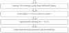
To obtain a stable and reliable clustering, we introduce a new clustering algorithm – Clustering System Based on Graphs (CSBG). CSBG uses a novel model involving a new graph representation. In explaining this model we use standard terminology of graph theory following, for example, the book [34] and the survey article [2009]. The flow chart of CSBG is presented in Figure 1 and is explained below in this section.
Let us denote the set of all patients from the DiabHealth database with ECG data used in our experiments by P = {p1, p2, …, pm}, where m is the number of patients. In order to divide these patients into groups, we used several independent clusterings and then combined their outcomes by applying our new CSBG algorithm. Our experiments compared the effectiveness of the CSBG procedure with several other methods presented in the next sections. In the rest of this section, we discuss CSBG algorithm for the case of two clusters considered in the current experiments.
To begin the operation of CSBG algorithm, we generated a collection of 100 independent random initial clusterings
C ={K1,K2,…,K100} .
They were generated using the well known clustering algorithms MeanShift [36] and KMeans [37] , implemented in Sage [38] via its Scikit-learn package [39,40]. To make sure that the collection (1) consists of independent random clusterings generated using initial points covering the space well, we ran each of these two clustering algorithms for 50 random values of their input parameters to obtain 50 different random clusterings for each clustering system. Then we combined all of these clusterings into the common collection C of 100 clusterings.
More specifically, the output of the MeanShift algorithm depends on the value of the input parameter ‘seeds’, which is used to initialise the iteration process. We ran MeanShift with 50 random values of the ‘seeds’ to ensure that it creates 50 different and independent output clusterings. Likewise, the output of KMeans algorithm depends on the selection of initial centroids. It is determined by the input parameters ‘init’, ‘n_init’ and ‘random_state’. We set the value of ‘init’ equal to the string ‘random’. This option makes KMeans to start with set initial centroids chosen randomly in the data set. We set the value of ‘n_init’ parameter equal to 1 to make KMeans output each random clustering immediately when it is obtained. The random selection process of initial centroids in KMeans depends on the value of the ‘random_state’ parameter, which is used every time as a seed to the random number generator incorporated in the algorithm. We ran KMeans 50 times with 50 different random values of the ‘random_state’ parameter to make sure that it generated independent random clusterings.
This means that for each value of i = 1, 2, …, 100, each particular clustering Ki comprises two clusters:
Ki = {Ki1, Ki2},
which partition the set P of patients so that the whole set P is a disjoint union of these clusters
P = Ki1∪Ki2.
CSBG procedure takes the collection C of 100 clusterings as input and produces a new common clustering
K = {K1, K2},
which also partitions the whole set P of patients
P = K1∪K2.
and at the same time achieves the best agreement with all the given clusterings K1, K2,…,K100.
CSBG procedure is based on a graph G = (V, E) illustrated in Figure 2. The set V of nodes of the graph G is a union of two subsets: V = Vp∪Vk. The number of nodes in the first subset Vp is equal to the number m of patients, so that Vp = {v1,v2,…,vm}. For i = 1, 2, …, m, the node vi serves as a graphical representation of the corresponding patient pi. The number of nodes in the second subset Vk is equal to 2 x 100 = 200, the number of clusters in all clusterings K1, K2, …, K100. Hence we get Vk = {v(m+1),v(m+2),…,v(m+200)}, where these nodes represent the corresponding clusters.
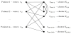
The set E of arcs of the graph G is also a union of two subsets: E = Ek∪Ep. The first subset Ek contains all arcs of the form (vm+2(j1)+l1, vm+2(j2)+l2 )), for all integers j1, j2, l1, l2 such that 0 ≤ j1< j2 ≤99 and 1 ≤ l1, l2 ≤ 2. This arc represents the following pair of clusters: the cluster K(j1+1)l1) of the clustering K(j1+1) and the cluster K(j2+1)l2) of the clustering K(j2+1). The weight of this arc is set equal to the Jaccard similarity index w(K(j1+1)l1),K(j2+1)l2), which measures the similarity of the clusters K(j1+1) l1) and K(j2+1) l2, and is defined by the formula
On the other hand, the subset Ep consists of all arcs of the form (vi,vm+2(j)+l), for all integers i, j, l such that 1 ≤ i ≤ m, 0 ≤ j ≤ 99, 1 ≤ l ≤ 2 and such that the patient pi belongs to the cluster Kjl of the clustering Kj. This means that the arcs of the subset Ep connect nodes representing patients to the nodes of the clusters where they belong.
We used spectral clustering available in Sage to partition the graph into two clusters. The final outcome of CSBG is then given by the way the spectral clustering partitions all nodes of the set corresponding to the patients. Note that the graph G=(V,E) is neither complete nor bipartite.
5. Other Classification and Clustering Systems
Our experiments compared the performance of CSBG with the following clustering systems available in Sage [38] , [40] : MeanShift [36] and KMeans [37] , Ward hierarchical clustering [42] , DBSCAN [43] , and Birch clustering systems [44] , for the diagnosis of severe CAN.
In addition, we also compared the performance of the CSBG procedure with Hybrid Bipartite Graph Formulation (HBGF) and Cluster-Based Graph Formulation (CBGF), which are two other clustering systems based on graphs proposed in [45] . Both of these procedures use smaller and simpler graphs. The number of arcs and nodes in these graphs and their structures are different from the graph in CSBG. For the case of m patients, two clusters and 100 initial clusterings the HBGF procedure uses a bipartite graph with m + 200 nodes and 100m arcs, and the CBGF uses a complete graph with 200 nodes. Thus, the graph used in the CSBG procedure has a different structure. We used our in-house C# implementation of these procedures. The readers are referred to [46=Yearwood 2009] for previous work in other research domains using HBGF and CBGF algorithms and further bibliography.
Furthermore, our experiments compared the outcomes obtained by CSBG with the results produced by several other classification systems available in Sage [38] via its package Scikit-learn [39,40]. This section presents classification and clustering systems being compared with CSBG.
DecisionTreeClassifier (DTC) incorporated in Sage, is a decision tree classification system using an optimised version of the Classification and Regression Trees (CART) algorithm. CART is similar to C4.5 classification system. However, it is capable of handling both classification and regression, and unlike C4.5 algorithm, it does not compute rule sets [38,40].
Sage provides three versions of the Naive Bayes algorithm: Gaussian Naive Bayes (GNB), Multinomial Naive Bayes (MNB), and Bernoulli Naive Bayes (BNB).
Nearest Centroid Classifier (NCC) available in Sage uses classes determined by centroids similar to the clusters of the classical k-means clustering system.
Sage includes two versions of Support Vector Machine (SVM) classification system: SVC and NuSVC. We used NuSVC with the default value 0.5 of υ parameter. They can operate with the following kernels: ‘linear’, ‘poly’, ‘rbf ’, ‘sigmoid’. To indicate the kernel being invoked we use the following notation: SVC[linear], SVC[poly], SVC[rbf], SVC[sigmoid], NuSVC[linear], NuSVC[poly], NuSVC[rbf], NuSVC[sigmoid].
Sage contains two versions of the well-known nearest neighbour classifier: KNeighborsClassifier (KNC) and RadiusNeighborsClassifier (RNC). KNC applies nearest neighbours. RNC applies all neighbours contained in a sphere of radius indicated by the user as a parameter. For DiScRi data, RNC algorithm produced substantially worse outcomes than KNC, and so we did not include RNC in the diagrams below.
RandomForestClassifier (RFC) is an efficient ensemble classification system available in Sage. It operates using one of two criteria measuring the quality of split of data: Gini Impurity or Information Gain. These options are specified by indicating the “criterion” parameter as “gini” or “entropy”, respectively. In the diagrams representing the results of our experiments these versions of RFC are denoted by RFC G and RFC-E, respectively. Furthermore, the number of trees in the forest can also be specified as the n_estimators parameter. In the diagrams representing the results of our experiments these classification systems with the number of trees equal to n are denoted by RFC G[n] and RFC-E[n], respectively.
For theoretical prerequisites and more detailed information on these classification systems the readers are referred to [38] , [40] and [41] .
6. Results and Discussion
Experiments presented in this article investigate the effectiveness of CSBG and other classification and clustering systems in their ability to diagnose of severe CAN. This means that these experiments looked at the binary classification with two classes: severe CAN and absence of severe CAN. We applied our new clustering approach CSBG and compared it with HBGF, CBGF and with other classification and clustering systems available in Sage [38] .
In testing the effectiveness of algorithms during our experiments, for each classifier we determined its F measure, precision, recall, sensitivity and specificity, see Section 5.7 of the book [41] for explanations of these notions. Our experiments have shown that all outcomes turned out consistent for the three data sets indicated in Table 1. This means that if the classifier achieved better results in terms of F measure, than it also obtained better precision, recall, sensitivity and specificity. Moreover, the histograms representing all of these metrics have the same shape and are quite similar. Therefore, to avoid duplication in representing the results, it suffices to include only the figures representing the F-measure of outcomes, since the corresponding diagrams for precision, recall, sensitivity and specificity look almost identical. In the diagrams with outcomes in this paper we include the F-measure, since it combines precision and recall into a single number evaluating performance of the whole system. It is a very well known metric often used in engineering research to evaluate the effectiveness of classification systems.
Here we include a succinct summary of the definition of F-measure with a discussion of precision, recall, sensitivity and specificity. The readers are referred to Section 5.7 of the book [41] for more details. The values of F-measure belong to the interval from 0 to 1. The very best value 1 means that the classifier predicted the values of all instances correctly. F-measure is defined as the harmonic mean of precision and recall
Precision of a classifier, for a given class, is the ratio of true positives to combined true and false positives. Recall is the ratio of true positives to the number of all positive samples (i.e., to the combined true positives and false negatives). The recall calculated for the class of patients with severe CAN coincides with the sensitivity of the whole classification systems, which is often used in medical research. Sensitivity is the proportion of positives (patients with severe CAN) that are identified correctly. It is also called the True Positive Rate (TPR). Specificity is defined as the proportion of people without severe CAN who have a negative test result. Weighted average values of these performance metrics are usually used. This means that they are calculated for each class separately, and a weighted average is then found. In particular, our results deal with the weighted average values of F-measure computed using the weighted average values of the precision and recall. The F-measure of a clustering system is defined by the same formula where each cluster is associated with the class of the majority of its elements. The values of precision, recall, sensitivity and specificity all belong to the same interval from 0 to 1, where the best value is 1 in terms of all of these metrics.
DiScRi is the largest known database with CAN information. It is the only database available for the authors of this paper. In order to use several data sets for more thorough evaluation of algorithms, we selected three samples from DiScRi database. These three data sets are used in all our experiments. They are described in Table 1.
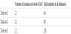
The largest data set 3 contains all patients in the DiabHealth database with complete available HRV features at the time of this work. We recorded all available demographic and clinical parameters for these patients in a csv file. To prepare data for the experiments we added Allan exponents. Data set 3 most closely represent real life data. The smallest data set 1 was created artificially to explore what happens when both classes of the severe CAN classification are perfectly balanced are have equal number of instances. Data set 2 plays an intermediate role. Besides, it may reflect the fact that the class ‘absence of severe CAN’ is in fact the union of three original Ewing classes, so that in an artificial data set it might make sense to allocate 3 times more instances to this class as compared to the class of patients with severe CAN.
Further, all our experiments used the standard and well known technique of 10 fold cross validation to avoid overfitting in evaluating the effectiveness of classification systems during the experiments, see [41] for more explanations.
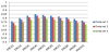
In order to compare the performance of CSBG with other systems available in Sage, we had to determine the best kernels to be used for SVC and NuSVC, and the best values of input parameters for several other systems in the case of diagnosing severe CAN. In Sage, SVC and NuSVC are available with four kernels: linear kernel, polynomial kernel, rbf kernel and sigmoid kernel. This means that each algorithm SVC and NuSVC can be executed invoking any of the four kernels. We refer to [40] for more information on the formulas used in these kernels and denote these versions of SVC and NuSVC by SVC[linear], SVC[poly], SVC[rbf], SVC[sigmoid], NuSVC[linear], NuSVC[poly], NuSVC[rbf], and NuSVC[sigmoid], respectively. First, we conducted tests to determine the performance of SVC and NuSVC with various available kernels. The F-measures obtained during this first set of experiments are presented in Figure 3.
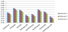
Figure 3 shows that in the diagnoses of severe CAN the best F-measure 0.79 was achieved by SVC with polynomial kernel. This outcome will be used to compare to the outcomes obtained by other systems below.
The KNC algorithm has an input parameter k, which is an integer specifying fixed number of nearest neighbours to be used in the algorithm. We use notation KNC[k] to indicate the value k as a parameter in the diagrams representing the results of our experiments. Figure 4 presents the F measures of the diagnosis of severe CAN obtained by KNC[k] for various values of the parameter k. We used KNC algorithm based on KDTree with uniform weights.
The best F-measure was obtained by KNC with k=4 (Figure 4). This result is included as the performance of KNC in the combined diagram below.
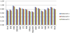
Next, we evaluated the performance of RFC-G and RFC-E algorithms for various options of the input parameter – the number of random trees. These values of F-measure are presented in Figure 5.
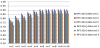
Figure 5 shows that the best value 0.86 of the F-measure was achieved by RFC G using six random trees after which results plateaued out. This option is also included for RFC in the combined diagram below.
Finally, the results of comparing CSBG to other graph-based clustering systems CBGF, HBGF and classification systems available in Sage are depicted in Figure 6. In this diagram we included the best available options determined above for the SVC, KNB and RFC algorithms.
The results of all experiments show that the best F-measure of 0.92 was obtained by the CSBG algorithm. Note that the ensemble classifier RFC implemented in Sage has achieved the very best performance among all classification and clustering systems readily available in Sage. It can also be recommended for practical assessment and the diagnosis of severe CAN.
7. Conclusions
This is the first paper concentrating on the diagnosis of severe CAN. This means considering the binary categorisation with two classes: severe CAN and absence of severe CAN. The innovations of this work included the introduction of a new Clustering System Based on Graphs (CSBG) and applying it for the diagnosis of severe CAN. Our experiments compared the effectiveness of CSBG to other clustering and classification techniques. The Allan exponents (AE) are scale-independent nonlinear HRV features applied in our experiments. The present article presents the results of experiments concentrating on the role of severe CAN and comparing the effectiveness of CSBG with the applications of other clustering systems and classification systems. The results demonstrate that our new procedure outperformed other techniques and obtained the best outcomes. The diagnosis of severe CAN by CSBG achieved the best performance level with F measure of 0.92 in the largest data set.
As options for future research we would like to suggest investigating supervised classification and clustering systems for the diagnosis of severe CAN. It would be also nice to examine the effectiveness of the CSBG system for different data sets available for experimental studies in other research domains.
Competing Interests
The authors declare that they have no competing interests.
Author Contributions
All authors have contributed to the design and development of experiments, and participated in writing the text of this article. All authors reviewed and approved the final manuscript.
Acknowledgments
The authors are grateful to the anonymous reviewer for a thorough report with many remarks which have helped to improve the article.