


1. Introduction
An electrodialysis (ED) processes is applied widely for saline water desalination. The ED processes are classified to a singlepass (continuous) process, a feed-and-bleed process and a batch process. Among these processes, the single-pass process is the most fundamental one, and the performance of the process is discussed from various points as follows.
Belfort and Daly [1] constructed optimization routine for a singlepass electrodialysis plant. The algorithm was applied to the Office of Saline Water test bed plant at Webster, South Dakota and compared the actual cost and operating conditions. Avriel and Zeligher [2] developed a mathematical model for preliminary engineering design and economical evaluation of a single-pass ED plant. Detailed cost computations were performed resulting in capital investment and annual operating costs. Lee et al. [3] developed a computer simulation program for describing a single-pass process and estimated investment and operation costs. Further, ED plant was designed and optimized in terms of overall costs and the different parameters. Moon et al. [4] investigated ionic transport across membranes based on the one- and two-dimensional single-pass ED modeling using the principles of electrochemistry, transport phenomena and thermodynamics. Fidaleo and Moresi [5] simulated mass transfer, mass balance, potential drop and limiting current density in a single-pass operation based on the Nernst-Planck equation. Sadrzadeh et al. [6] modeled continuous flow desalination starting from a differential equation of steady-state mass balance and gives salt concentration in dilute compartments or separation percent for various voltages, flow rates and feed concentrations. Nikonenko et al. [7] described ED or electrodeionization characteristics (mass transfer coefficient, Sherwood number, degree of desalination and others). The reasonability of the functions was discussed with experimental measurements. Brauns et al. [8] developed a simulation model through solver software. Experimental verification of the software was performed using an industrial type pilot plant. Limiting current density was theoretically evaluated in the model calculations for design purposes and corrected with the experimental results.
The single-pass program becomes the basis of the feed-and-bleed program [9] and the batch program [10]. This is because the singlepass program describes the function of the electrodialyzer. This article describes the single-pass program established based on the principles of electrochemistry and ED experiments being supplied strong electrolyte solutions [11]. Calculation is carried out in the spread sheet with a use of common software (Excel) and ordinary hardware (Computer). The program is integrated in websites. So, readers can operate the program in the websites (Attached section) by inputting the source codes i.e. optional process specifications and operating conditions. The program aims to function as a pilot plant operation.
2. Single-pass ED Process
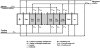
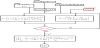
The one-stage single-pass (continuous) ED process is illustrated in Figure 1. The electrodialyzer is incorporated with desalting cells, concentrating cells in the stack marked with gray. Number of cells is N for desalting cells and N+1 for concentrating cells. The anode and cathode cells are placed at both outsides of the stack and an electric current is supplied between the electrodes. A feeding solution of salt concentration C’in is supplied to desalting cells at linear velocity of u’in at the inlets. C’in and u’in are decreased to respectively C’out and u’out at the outlets of desalting cells. A part of the feeding solution is also supplied to concentrating cells for preventing scale formation in the concentrating cells. The salt concentration and linear velocity in concentrating cells are respectively C’in = C’in and u”in at the inlets and C”out and u”out at the outlets. Partition cells are incorporated between the stack and electrode cells for preventing the influence of electrode reactions to the performance of the electrodialyzer. A part of a concentrated solution flowing out from the outlets of concentrating cells is supplied to electrode cells and partition cells. A multi-stage ED process is formed by arranging the single-pass process in Figure 1 in series.
3. Mass Transport in the Single-pass Process
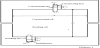
Figure 2 illustrates the mass transport in the single-pass (continuous) process. A salt solution (raw salt solution, concentration: C’in) is supplied to the inlets of desalting cells (De) at average linear velocity of u’in. For preventing scale formation in concentrating cells, a part of a raw salt solution is supplied also to the inlets of concentrating cells (Con) at the average linear velocity of u”in. By supplying an electric current I, ions and solutions are transferred from desalting cells to concentrating cells across an ion exchange membrane pair and their flux is defined by JS and JV respectively. In desalting (concentrating) cells, salt concentration is decreased (increased) along the flowpass from C’in (C”in = C’in) under applied average current density I/S and reaches average salt concentration C’out (C”out) at the outlets of desalting (concentrating) cells. Salt concentration change in desalting cells causes current density change along the flow-pass from iin at the inlets to iout at the outlets. The current density becomes j at x distant from the inlets of desalting cells. I/S, JS, JV, C’p, C”p, u’p and u”p are altogether the values at x = pl distant from the inlets of desalting and concentrating cells. Vin, Vout and Vp are voltage difference between electrodes respectively at the inlets (x = 0), the outlets (x = l) and x = pl of desalting cells (Vin = Vout = Vp).
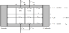
Figure 3 illustrates the desalting cell and concentrating cell.
4. Specifications and Operating Conditions of an Electrodialyzer
(1) Flow-pass thickness in a desalting and a concentrating cell; a (cm)
(2) Flow-pass width in a desalting and a concentrating cell; b (cm)
(3) Flow-pass length in a desalting and a concentrating cell; l (cm)
(4) Membrane area; S = bl (cm2)
(4) Number of stacks in an electrodialyzer; 1
(5) Number of desalting cells, concentrating cells and membrane pairs
integrated in a stack; N, N+1, N
(6) Probe electrodes are inserted into concentrating cells integrated at
the ends of a stack for measuring cell voltage
(7) Average current density; I/S (A/cm2)
(8) Salt concentration at the inlets of desalting cells ; C’in (eq/cm3)
(9) Salt concentration at the inlets of concentrating cells ; C’in = C’in
(eq/cm3)
(10) Linear velocity at the inlets of desalting and concentrating cells;
u’in, u”in (cm/s)
(11) Standard deviation of the normal distribution of solution velocity
ratio; σ
(12) Flow system in desalting and concentrating cells; single-pass flow
(13) Diagonal net spacers are integrated in desalting and concentrating
cells and in desalting and concentrating slots. Dimensions of a spacer
are:
Diameter of a spacer rod dS = half thickness of the cell; a/2
Distance between the rods; χ
Crossing angle of the rods; θ
| Number | thickness | width | length | |
| Desalting cell | 1 | a | b | l |
| Concentrating cell | 1 | a | b | l |
| Desalting slot and duct | n' | a | w' | h' |
| Concentrating slot and duct | n" | a | w" | h" |
5. Electrodialysis Program
Computing processes are explained definitely in the book ”Ion Exchange Membranes. Fundamentals and Applications 2nd edition” [12]. This section summarizes the specifications of the program briefly.
5.1 Overall mass transport equation
Fluxes of ions JS and a solution JV across an ion exchange membrane pair at x = pl distant from the inlets of desalting and concentrating cells are expressed by the following overall mass transport equation [13].
JS =λ(I/S) – μ(C”p – C’p) = (tK + tA -1) (I/S)/F – μ(C”p – C’p) = η (I/S)/F
JV = φ(I/S) + ρ(C”p – C’p)
in which λ (eqC-1) is the overall transport number, μ (cm s-1) is the overall solute permeability, φ (cm3C-1) is the overall electro-osmotic permeability and ρ (cm4eq-1s-1) is the overall volume osmotic permeability. t is the transport number of counter-ions in the membrane. η is the current efficiency and F is the Faraday constant.
ρ versus λ, μ and φ plots are given by the following empirical equations.
λ = 9.208×10⁻⁶ + 1.914×10⁻⁵ρ
μ = 2.005×10⁻⁴ρ
φ = 3.768×10⁻³ρ0.2 – 1.019×10⁻²ρ
ρ versus alternating current electric resistance of an ion-exchange membrane pair ralter = ralter,K + ralter,A is expressed by the following equation [14].
ralter = ralter,K + ralter,A = 1.2323ρ-(1/3)
The relationship between ρ and solution temperature T(⁰C) is approximated by the following equation [15].
ρ = 3.421×10⁻³ + 3.333×10⁻⁴T
Eqs. (3) – (6) mean that ρ is the leading parameter and it represents all of the overall membrane characteristics. λ, μ, φ, ralter,K+ratler,A and ρ are determined by setting T in Eq. (7). Eqs. (3) – (7) are empirical equations developed using electrodialyzers integrated with commercially available homogeneous ionexchange membranes and supplying inorganic strong electrolyte solutions. The equations are practically applicable under the above situations.
Membrane pair alternating electric resistance ralter is calculated using the following equations [14].
ralter = 1.2323ρ-1/3
Ion-exchange membranes usually work under a direct electric current. The direct current electric resistance of the membrane rdire = rmemb is influenced by the salt concentration of the solutions placed on both sides of the membrane, and it is expressed by the following equation [16].
where
κ’ and κ” are the specific conductivity of the solutions in a desalting cell and a concentrating cell respectively.
5.2 Feeding solution
Feeding solutions are limited to strong electrolyte solutions such as seawater, diluted seawater, concentrated seawater etc. Physical properties such as density, viscosity, specific conductivity, activity coefficient of the solution are expressed by the functions of electrolyte concentrations and temperature.
5.3 Salt concentration and linear velocity in desalting cells
Salt concentration and linear velocity at the inlets of the cells are set up freely. The solution velocity ratio ξ in desalting cells integrated in a stack in an electrodialyzer is defined by Eq. (12):
where u* is the linear velocity in every desalting cell and u̅ is the average linear velocity in a stack. The frequency distribution of ξ is expressed by the normal distribution. Thus the minimum of ξ and u* is equated with –3σ and u, respectively, where σ is the standard deviation of the normal distribution of ξ and u is the minimum value of linear velocities within all desalting cells in a stack. Putting ξ = -3σ and u* = u in Eq. (12) yields Eq. (13):
u = u(1-3σ)
σ = 0.1 is assumed in the program taking into account the experimental results. σ affects on the limiting current density and functions as a safety parameter to operate an electrodialyzer. σ does not exert an influence to the performance of an electrodialyzer excepting the limiting current density.
5.4 Current density distribution
In an ED system, current density is decreased due to the salt concentration decrease in desalting cells along a flow-pass. This phenomenon have a effect on the limiting current density of an electrodialyzer (I/S)lim. The current density distribution is assumed to be approximated by the following quadratic equation expressed at x/l distant from the inlet of a desalting cell.
To determine a1, a2 and a3 in Eq. (14), three simultaneous equations are set up [17,18](Tanaka, 2000, 2002) assuming voltage differences between electrodes are constant and independent of x/l.
5.5 Limiting current density
When current density reaches the limit of a cation-exchange membrane ilim at the outlet of a desalting cell in which linear velocity becomes the least among u’in; u’in# , the average current density applied to an electrodialyzer is defined as its limiting current density (I/S)lim which is expressed by Eq. (15).
in which, C’out# is C’out at u’ = u’in# which is given by:
u’in# = u’in(1 – 3σ)
σ is the standard deviation of the normal distribution of solution velocity ratio ξ, and it is defined in Eq. (13).
5.6 Salt concentration and linear velocity in concentrating cells
Salt concentration and linear velocity at the inlets of concentrating cells are set up freely and those at the other positions (0 < x/l < 1) are calculated from the material balance.
5.7 Electric resistance of a desalting and a concentrating cell
Electric resistance of a desalting cell r’ and of a concentrating cell r” in an electrodialyzer are given as:
ε defines an electric current screening effect of a diagonal net spacer and it is determined by the volume ratio of spacer rods in a desalting and concentrating cell as follows.
in which χ is the distance between spacer rods, θ is the crossing angle of the rods.
5.8 Cell voltage, energy consumption, water recovery and desalting ratio
Ohmic voltage and membrane voltage at the inlet of the desalting cell (VΩ,in and Vmemb,in) and those at the outlet of the desalting cell (VΩ,out and Vmemb,out) are:
in which, j stands for group j in the normal distribution.
Cell voltage Vcell is introduced from Eqs. (21) - (23) as shown in Figure (24).
Vcell (V/pair) = VΩ,in + Vmemb,in = VΩ,out + Vmemb,out
Energy consumption E is expressed by the following equation.
q’out is the solution volume; output of the desalted solution (cm3/s cell).
Water recovery Re is:
Desalting ratio α is:
5.9 Pressure drop in desalting and concentrating cells and slots
Hydrodynamic diameter of a desalting or a concentrating cell (electric current passing section); dH,cell and that of a desalting or a concentrating slot; dH,slot incorporated with a diagonal net spacer are expressed by the following equation [19,20].
in which w is the flow-pass width in the slot (Figure 3).
Pressure difference between the inlet and the outlet of the cell in a desalting or a concentrating cell; pressure drop in the cell (in the electric current passing section) ΔPcell and that in a desalting or a concentrating slot; pressure drop in the slot ΔPslot are [20].
in which, h is the flow-pass length in the slot (Figure 3), ucell is linear velocity in the desalting or concentrating cell, uslot is linear velocity in the slot. μ (g cm-1s-1) is the viscosity coefficient of a solution. ucell and uslot are linear velocity in the cell and slot. ΔP (m) is calculated using ΔP (m) = 1.01972×10⁻⁴ΔP(Pa).
5.10 Elecric current leakage
In an electrodialyzer, a part of an electric current does not pass through ion-exchange membranes and it flows between electrodes through slots and ducts. Electric current leakage is an ineffective and inevitable phenomenon which increases energy consumption in an ED process. Leakage current ratio IL/I0 is introduced by Wilson [21] as follows.
where Rs* is the overall slot electric resistance and Rd* is the overall duct electric resistance defined as follows.
in which R is the electric resistance of a cell pair and
5.11 Structure of a desalting cell, concentrating cell, slot and duct and cell pair number.
The following parameters are set up freely.
Thickness a , width b and length l of a desalting and a concentrating cell; Cell pair number N;
Structure of a diagonal net spacer, a slot and a duct.
5.12 Units in the program
The program consists of empirical equations and principles of electrochemistry. It is developed fundamentally based on the SI units with prefixes. In order to apply the program to industrial operation, the units are suitably converted to industrial units such as kWh/m3, m3/h, A/dm2, mg/dm3 = ppm etc. Thus the units are substantially mixed and not unified.
6. Program
The program is developed based on fundamentally the equations described in Section 5. The single-pass ED process is classified as follows.
(1)Constant current single-pass process
(2)Constant voltage single-pass process
(3)Constant salt concentration single-pass process
Among the above processes, the constant voltage single-pass process is widely applied because the ED operation is carried out stably. Figure 4 shows the constant voltage single-pass program. The computation is carried out through three steps.
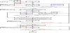
(1) Step 1 (Computer operation time; 5 min)
Decision point 1 ()
I* (Control key 1) is adjusted to equalize Vcellinput with computed Vcell as follows.
Vcellinput = Vcell
Decision point 2 ()
C’p* and C”p* (Control key 2) are equalized to computed C’p and C”p for preventing circulation reference as follows
C’p* = C’p C”p* = C”p
Decision point 3 ()
p* (Control key 3) is adjusted to realize
ζinout = ζinp
(2) Step 2 (Computer operation time; 2 min)
Decision point 4 ()
I#* (Control key 4) is adjusted to realize
I#*(1 – IL/I#*) = I
(3) Step 3 (Computer operation time; 2 min)
In the limiting current density program (Figure 5), control key C’out#*
is adjusted to realize
Z1 = Z2
where C’out#* is C’out at u’in = u’in# given by Eq. (16).
7. Computation
The program is integrated in the website. So, readers can operate the program in the website (Attached section) by inputting the source codes i.e. optional process specifications and operating conditions.
8. Specifications and operating conditions of an electrodialysis process
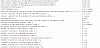
Table 1 lists the standard process specifications and ED conditions. The process performances are computed by changing cell voltage Vcell incrementally.
9. Results
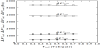
Ion flux JS and solution flux JV are plotted against Vcell (Figure 6). Current density I/S and energy consumption E are plotted against Vcell (Figure 7). I (A) is the total electric current and S (cm2) is the effective membrane area, thus I/S is the average current density. Figure 8 shows the salt concentration at the outlets of desalting cell C’out and the outlets of concentrating cells C”out, desalting ratio α, water recovery Re and current efficiency η.
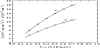
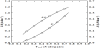
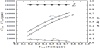
Figure 9 is the limiting current density diagram in which the limiting current density (I/S)lim and Vcell are plotted against I/S. The real limiting current density of the electrodialyzer (I/S)lim,real is determined from the intersection between the (I/S)lim line and the I/S = (I/S)lim line as (I/S)lim,real = 1.135 A/dm2. From this point, the limiting cell voltage Vcell,lim = 0.696 V/pair is presumed.
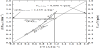
Figure 10 gives the current density distribution; i = a1 + a2(x/l) + a3(x/l)2. i is local current density at x/l. x/l = 0 and x/l = 1 correspond to respectively the inlet and the outlet of desalting and concentrating cell. i becomes the average current density I/S at x/l = p which is shown by the point (p, I/S) in the figure.
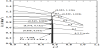
Figure 11 shows Vcell versus p, r’, r”, rmemb and IL/I. Here, r’, r” and rmemb are respectively the electric resistance of the solution in the desalting cell, in the concentrating cell and the direct electric resistance of a membrane pair at x/l = p. IL/I is the electric current leakage. With the increase of Vcell'r” is decreased, however, r’, rmemb and IL/I are increased. When Vcell is decreased toward zero, p is seen to be decreased after passing through the maximum value.
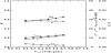
Figure 12 shows total pressure drop in the desalting side ΔP’total and in the concentrating side ΔP”total, and pressure drop in the electric current passing portion in the desalting cell ΔP’cell and in the concentrating cell ΔP”cell. The pressure drop in the slot in the desalting cell and in the concentrating cell ΔPslot is equivalent to the total pressure drop at the inlet and outlet; ΔPslot = ΔPslot,inlet + ΔPslot,outlet and it is calculated from Pslot = ΔPtotal - ΔPcell .
10. Attached Section
10.1 Computing steps in the program in the website
10.1.1 A1 Website
The website is established based on the stand alone ED program. This section describes “Constant voltage single-pass (continuous) program” integrated in the website.
10.1.2 A2 Steps in the program computation
The program is written in the Excel spread sheet, and it consists of the
following 11 steps.
Step 1 Fundamental specifications of an electrodialyzer and operating
conditions
Step 2 Fundamental operating conditions of an electrodialyzer
Step 3 Solution electric resistance and salt activity coefficient in
concentrating cells
Step 4 Solution electric resistance and salt activity coefficient at the
inlets of desalting cells
Step 5 Computation at Vin = Vout
Step 6 iin, iout, ohmic voltage, membrane potential, cell voltage, energy
consumption
Step 7 Computation at Vin = Vp
Step 8 p, ζin, ζout, a1, a2 and a3
Step 9 Solution viscosity and pressure difference in desalting cells and
concentrating cells
Step 10 Electric current leakages
Step 11 Limiting current density
10.1.3 A3 Remarks in the program computation
(1) Calculations in the decision points are marked with . Inputs are
marked with . Important values are marked with .
(2) Readers can operate the program by inputting the optional input
() and carrying out the trial-and-error calculations at the
decision points () as follows (cf. Figure 4 and Section 6).
Decision point 1
Control key 1; I*
Adjust I*/S to realize Vcellinput = Vcell
Decision point 2
Control key 2; C’in*, C”in*
Adjust C’p* and C”p* to realize C’p* = C’p and C”p* = C”p
Decision point 3
Control key 3; p*
Adjust p* to realize ζinout = ζinp
Decision point 4
Control key 4; I#*
Adjust I#* to realize I#*(1 – IL/I#*) = I
Limiting current density
Control key; C’out#*
Adjust C’out#* to realize Z1 = Z2
(4) Summary is supplied at the end of the spread sheet for printing.
Competing Interests
The author declare that he has no competing interests.