


1. Introduction
In a randomized trial to compare two groups where the outcome is binary, the results can be summarized into a two-by-two contingency table and the equality of the response proportions between the two groups compared using a statistical hypothesis test.
Two widely used tests that make such a comparison and do not require any approximations are Fisher’s exact test [1,2] and Barnard’s exact test [3-5]. The former is more popular than the latter; however, Barnard’s exact test has advantages over Fisher’s exact test in that it is more powerful for moderate to small samples [6]. Although until recently it was not applied because of the significant computation time needed for the numerical search, it can now be applied easily using a software package such as SAS. Recently, Chiba [7] developed new exact tests; i.e., a conditional exact test, in which one marginal total is fixed, and an unconditional exact test, in which neither marginal total is fixed. Fisher’s exact test can be regarded as a special case of Chiba’s conditional exact test. The confidence intervals (CIs) linking to Barnard’s and Chiba’s exact tests can be constructed in a straightforward manner.
In this article, we review these three exact tests by noting the differences in the null hypotheses that they test. Furthermore, using a simple numerical example, we demonstrate that the CI linking to Barnard’s exact test is not in fact an exact CI for the causal effect. For this demonstration, we apply the nonparametric bounds [8,9].
2. Notation and Principal Stratification
We use the following notation through this paper. Let X denote the assigned treatment; X = 1 if a subject was assigned to the treatment group, and X = 0 if assigned to the control group. Let Y denote the binary outcome; Y = 1 if the event occurred, and Y = 0 if it did not. Finally, let Y(x) denote the potential outcomes [10] for each subject under X=x, which corresponds to the outcomes of the subject had he/ she been in the trial group. Then, Pr(Y(x) = 1) represents a potential response proportion if all subjects are assigned to the group with X = x.
Here, we apply the principal stratification approach [11]. This approach considers the following four types of subjects to define the four principal strata:
- Individuals for whom the event would occur regardless of the assigned treatment group; i.e., (Y(1), Y(0)) = (1, 1).
- Individuals for whom the event would occur if assigned to the treatment group but would not occur if assigned to the control group; i.e., (Y(1), Y(0)) = (1, 0).
- Individuals for whom the event would not occur if assigned to the treatment group but would occur if assigned to the control group; i.e., (Y(1), Y(0)) = (0, 1).
- Individuals for whom the event would not occur regardless of the assigned treatment group; i.e., (Y(1), Y(0)) = (0, 0).
All subjects belong to one of these four types; however, unfortunately we cannot know the numbers of type (i)–(iv) subjects from the observed data.
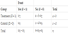
To review the three exact tests, let us assume that the generic twoby- two contingency table in Table 1 is obtained from a randomized trial, where a, b, c, d, and n are the numbers of subjects. The risk difference can be calculated as follows:
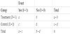
Here, we consider the case of RDO≥ 0, but a similar discussion holds for the case of RDO≤ 0. Table 2 lists simple example data for a hypothetical randomized trial with the assignment ratio of 1:1, RDO = 3/5 – 1/5 = 0.4.
3. Review of Exact Tests
3.1 Fisher’s exact test
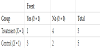
Let us denote a generic two-by-two contingency table under the null hypothesis using random variables W1 and W0 such as in Table 3. Here, the null hypothesis for Fisher’s exact test is as follows:
H0: Y(1) = Y(0) for all subjects,
which is referred to as the sharp causal null hypothesis [12].
Under this null hypothesis, subjects are limited to those with (Y(1), Y(0)) = (0, 0) or (1, 1), which implies that an outcome for a subject is constant regardless of the assigned group. Then, subjects with Y = 1 are those with(Y(1), Y(0)) = (1, 1), and similarly subjects with Y = 0 are those with(Y(1), Y(0)) = (0, 0). Therefore, under the sharp causal null hypothesis, w0 + w1 = a + c and n–w0–w1 = b + d from Tables 1 and 3.
The probability of W1 = w1 under the sharp causal null hypothesis is given by the hypergeometric distribution as follows:
where and max {0, a–d} ≤ w1≤ min {a + b, a + c}. This is the probability that w1 subjects of (a + c) subjects who experienced the event, and (a + b–w1) subjects of (b + d) subjects who did not experience the event are selected in the treatment group, when (a + b) subjects of the total n subjects are selected in the treatment group.
Because the risk difference under the null hypothesis can be expressed as
the one-sided p-value can be calculated by
where I(z) := RDN– RDO = 1 if z≥ 0 and I(z) = 0 if z< 0 with z = RDN– RDO. The second equation is derived because w0 = a + c–w1 and thus
This is the p-value for Fisher’s exact test. For the hypothetical data listed in Table 2, we have
3.2 Barnard’s exact test
Let the response probability for the group with X = x be Pr(Y = 1 | X = x) = πx. Then, the probability of observing w1 and w0 is given by the following product of two binomial probabilities:
The null hypothesis for Barnard’s exact test is as follows:
H0: π1 = π0.
Therefore, for π1 = π0 = π, the one-sided p-value can be calculated by
Unfortunately, because this calculation of the p-value includes a nuisance parameter π, we cannot yield the p-value immediately. Thus, we yield the p-value by calculating the p-values for all possible π and choosing the maximum value; i.e., p = sup{pπ}. This is the p-value for Barnard’s exact test. For the hypothetical data in Table 2, we have
An SAS program to yield the p-values for Fisher’s and Barnard’s exact tests is given in the appendix.
3.3 Chiba’s exact test
Let nst denote the number of subjects with (Y(1), Y(0)) = (s, t), where s, t = 0, 1. If all subjects are assigned to the treatment group (X = 1), then Pr(Y(1) = 1) = (n11 + n10) / n, because only subjects with type (i) or (ii) would experience the event. Likewise, if all subjects are assigned to the control group (X = 0), then Pr(Y(0) = 1) = (n11 + n01) /n, because only subjects with type (i) or (iii) would experience the event.
The null hypothesis for Chiba’s exact test is as follows:
H0: n10 = n01.
This null hypothesis corresponds to Pr(Y(1) = 1) = Pr(Y(0) = 1), which is referred to as the weak causal null hypothesis [12].
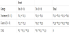
Let us assume that of the nst subjects, nst,1 subjects were assigned to the treatment group (X = 1), and nst,0 subjects were assigned to the control group (X = 0) by random assignment at a 1:r ratio. This leads to the two-by-two contingency table shown in Table 4. Applying the binomial probabilities, the one-sided p-value can be calculated by
where I'(Z)=1 if z≥ 0 and I'(Z)=0 if z< 0 with , z=RD'N- RDO and
where nst (s, t = 0, 1) must satisfy the following conditions:
Similar to Barnard’s exact test, because this calculation of the p-value includes the nuisance parameters n11, n10, n01 and n00, we cannot yield the p-value directly. Thus, we yield the p-value by calculating the p-values for all possible combinations of (n11, n10, n01 and n00) and choosing the maximum value; i.e., p = sup{ pn11,n10,n01,n00}. This is the p-value for Chiba’s unconditional exact test. For the hypothetical data in Table 2, we have
For Chiba’s conditional exact test,
is applied rather than (1), and ΣsΣtnst,1 = a + b is added to the conditions in (2). As with Fisher’s exact test, the calculation of this p-value is based on the probability that nst,1 subjects of nst subjects are selected in the treatment group when (a + b) subjects of the total n subjects are selected in the treatment group. Note that the special case of n10 = n01 = 0, for which subjects are limited to those with (Y(1), Y(0)) = (0, 0) or (1, 1), corresponds to Fisher’s exact test. For the hypothetical data listed in Table 2, we have
4. Difference in Null Hypotheses
Table 5 lists the null hypotheses for the three exact tests. In many actual randomized trials, the most interesting null hypothesis will be the weak causal null hypothesis, where the causal risk difference is zero; i.e., Pr(Y(1) = 1) – Pr(Y(0) = 1) = 0. Chiba’s exact test is a hypothetical test for the weak causal null hypothesis; however, Fisher’s and Barnard’s exact tests are not. The weak causal null hypothesis holds whenever the sharp causal null hypothesis holds, but rejection of the sharp causal null hypothesis does not imply rejection of the weak causal null hypothesis; i.e., Pr(Y(1) = 1)–Pr(Y(0) = 1)≠ 0 [7]. Barnard’s exact test includes nothing about the causal effect.
Nevertheless, Fisher’s exact test can be a hypothesis test for the weak causal null hypothesis under the monotonicity assumption [13,14], which implies that there are no subjects with (Y(1), Y(0)) = (0, 1). Barnard’s exact test can be a hypothesis test for the weak causal null hypothesis under the exchangeability assumption [15], which implies that, in a randomized trial with a 1:1 ratio, the number of type (i)–(iv) subjects in the treatment group is exactly equal to that in the control group. See Chiba [7] for further details.
5. Exact Confidence Intervals
We can construct the exact CIs linking to Barnard’s and Chiba’s exact tests, whereas the exact CI linking to Fisher’s exact test cannot be constructed in a straightforward manner. Specifically, the exact CI linking to Barnard’s exact test can be yielded easily using the FREQ procedure in SAS (version 9.4, SAS Institute, Cary, NC, USA). The program used to achieve this is described in the appendix.
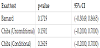
We applied the exact CIs to the data listed in Table 2. The 95% CIs are given in Table 6, where the risk difference was –0.4.
To examine whether these CIs are in fact exact CIs for the causal effect, we applied nonparametric bounds [8,9]. Nonparametric bounds are a range within which the causal risk difference must exist and are given by
–{Pr(Y = 1, X = 0) + Pr(Y = 0, X = 1)}
≤ Pr(Y(1) = 1)–Pr(Y(0) = 1)
≤ Pr(Y = 1, X = 1) + Pr(Y = 0, X = 0).
For the hypothetical data in Table 2, we have
–(1/10 + 2/10) = –0.3
≤ Pr(Y(1) = 1)–Pr(Y(0) = 1)
≤ (3/10 + 4/10) = 0.7.
Since the nonparametric bounds describe a range within which the causal risk difference must exist, the upper limit of 95% CI must be smaller than the upper nonparametric bound, and the lower limit must be larger than the lower nonparametric bound. However, for the CI linking to Barnard’s exact test, the upper limit (0.8665) was larger than the upper bound of 0.7, and the lower limit (–0.3049) was smaller than the lower bound of –0.3. This demonstrates that the 95% CI linking to Barnard’s exact test includes values that the causal risk difference cannot take. As a consequence, the exact CI is not in fact an exact CI for the causal effect. Barnard’s exact test is exact for Pr(Y = 1 | X = 1) – Pr(Y = 1 | X = 0) but not for the causal effect Pr(Y(1) = 1) – Pr(Y(0) = 1). The limits of the CIs linking to Chiba’s exact test cannot be outside the nonparametric bounds, because the inequalities in (2) correspond to the nonparametric bounds.
6. Discussion and Conclusion
We have reviewed three exact tests for two-by-two contingency tables in the context of randomized trials and demonstrated that the exact CI linking to Barnard’s exact test is not in fact an exact CI for the causal effect.
Researchers may encounter a situation in which they would like to examine the weak causal null hypothesis but cannot apply a hypothesis test for it. In such a situation, we recommend that they employ Fisher’s exact test when the sample size is small, for the following two reasons. First, we have a higher violation possibility of the exchangeability assumption for a relatively small sample size. Second, violation of the monotonicity assumption (i.e., at least one subject with (Y(1), Y(0)) = (1, 0) exists in the trial) will not be guaranteed for a small sample size. Conversely, in the case in which monotonicity cannot be assumed, we recommend that researchers employ Barnard’s exact test when the sample size is large, because it will not be claimed that exchangeability holds at least approximately. In general, Barnard’s exact test is more powerful than Fisher’s exact test for moderate to small samples [6]. Therefore, this recommendation will derive a conservative result. Nevertheless, such a result may be welcomed in randomized trials to avoid a large probability of type I error.
As demonstrated in the case with a small sample size, the CI linking to Barnard’s exact test was not in fact an exact CI for the causal effect. Therefore, we recommend that researchers do not apply this exact CI for small sample sizes.
In many randomized trials, the most interesting null hypothesis will be the weak causal null hypothesis. Nevertheless, to the best of our knowledge, exact tests for it have received little investigation. Such exact tests and CIs linking to them should be investigated further and applied to actual randomized trials.
7. Appendix
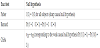
The following is an SAS program used to yield the p-values from Fisher’s and Barnard’s exact tests, as well as the exact CI linking to Barnard’s exact test.
data dat0;
cards;
1 1 3
1 0 2
0 1 1
0 0 4
run;
exact Barnard riskdiff (method=score);
weight count;
Competing Interests
The author declare that there is no competing interests regarding the publication of this article.