


1. Introduction
This 3-axis FVM urban landfill case study compares a low-level UAV survey with a ground survey to test if the UAV survey can reasonably approximate a ground survey’s resolution. Some of the following material is taken from Microsoft PowerPoint slides that were publicly presented by the author at two previous conferences [1,2]. Some of the content, though not all, was also presented, in modified or unmodified form, in a prior publication by the author [3]. The latter reference [3] also contains content, materials and findings not presented in this work.
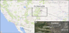
The Colorado landfill survey area is shown in Figure 1a and the Golden municipality survey site is pointed out by the white arrow, in the Landsat imagery figure inset 1b. The landfill site contains mappable buried and surficial ferromagnetic objects [4].
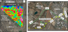
The two FVM surveys cover approximately 15 line-km on 10-meter (m) spaced E-W traverse lines (Figure 2a) and is outlined by the dashed red triangle in Figure 2b; the ground survey is followed by the low-level UAV survey. Both survey results are subsequently compared with a ground AVM third survey, that acts as the gridded TMI data image benchmark. There are several 60 Hz electromagnetic noise sources (EMI) in the area (Figure 2b) including 230 kV power lines on 30 m tall towers and a rail terminal with 750 V electrified tracks (yellow traces), 600 V roadside electrical lines (green traces), and several 120 and 240 V electrified buildings including an amusement park.
2. Materials and Methods
The UAV FVM survey (Figure 3a) employs a “FGM3D75 Magdrone” [5] system mounted on a Matrice 200 quadcopter [6]. The same FVM is used for both the ground and UAV surveys. Both the FVM and benchmark AVM “GSMP-35G” [7] ground survey sensors are mounted at 2 m height, using the same backpack during separate traverses on different days (Figure 3b). A second duplicate AVM is used as a base station for all surveys, to correct daily geomagnetic background variations (diurnals) for both FVM and AVM field data.
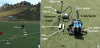
The FVM is scalar calibrated daily through a 360⁰ sphere using a technique that minimizes sensor movement, site gradient, active geomagnetic background and surveyor effects for both ground and UAV surveys. The UAV survey is flown over the landfill’s 15 km flight lines within a 2 to 6 m flight-height-envelope with the sensor an average 3 to 4 m height off the ground to approximate the 2 m ground traverse sensor height whilst maintaining safe clearance above sensorsnagging vegetation, primarily 2 to 3 m tall bushes scattered across the survey area.
A 1 m resolution LiDAR topographic image [8] (USGS LiDAR site, 2020) provides the flight control terrain drape surface. Standard GNSS Z-coordinate software settings then locate the slung sensor at an average 3 to 4 m height above the LiDAR surface, that acts as a terrain proxy. The FVM surveys test if a low-level UAV survey can replace a ground survey in first-pass reconnaissance circumstances. It will also test if ground calibrated FVM sensors, that are slung far enough below and isolated from the noise field of a UAV, can return higher quality airborne TMI data in a 60 Hz EMI-noise-contaminated urban environment.
3. FVM Sensor Calibration, Correction and Compensation
FVM field calibration prior to flights, that subsequently generate vector corrections, return lower noise levels and higher accuracy calculated TMI data from the three measured vector magnitudes. Studies in the 1950s began addressing the problems of compensation for fixed-wing aircraft platform noise in airborne magnetometer survey data, with [9] and [10]. A few years later [11], following a different calibration and compensation path, began research on the determination of satellite attitudes using a 3-axis FVM least squares fitting approach. She [11] and others furthered the attitude work, with later research including orbital FVM and scalar magnetometry; a few other but not exhaustive satellite FVM calibration examples include [12-15]. The satellite scientists use linear algebra matrices including singular value decomposition (SVD) and other formulations for FVM calibration and compensation. More recent satellite-derived formulations have been applied to UAV FVM surveying; three examples include [16-18]. The reference [16] discusses how their matrix formulation is equivalent to the quadratic polynomial compensation formulation in [10].
An outline of the 3-axis vector ellipsoid and spheroid fitting and correction method is seen in Figure 4, with a simplified SVD matrix formulation that was presented in [1,2] with ellipsoid, spheroid and vector graphics modified from [19]. The uncalibrated (raw) readings (BR) are represented by the ellipsoid and its distorted vectors. After calibration and subsequent vector correction determinations, the distorted ellipsoid is transformed into the compensated spheroid result (BC), where the vector origins (OO offsets) are translated to the sphere centroid, rotated to 90⁰ orthogonality for the three axes (A vectors), and scaled to the background norm (S vectors) that at the landfill was approximately 52,000 nT, as will be seen in some following figures.
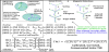
The ground calibration procedure corrects the FVM sensor for manufacturing errors prior to being slung below the UAV. A compensation for platform-sourced magnetic distortions at the sensor, could also be corrected for, if the sensor were mounted in a fixed orientation on the platform, using an airborne calibration flight. The second set of vector corrections for permanent hard iron (OI) and induced soft iron (SI and AI) and magnetic eddies (E) would apply also, if the FVM sensor was in the UAV noise field. As the slung FVM sensor is isolated from the UAV noise, an airborne calibration is not required, as reviewed in the following noise test section. A general discussion of the SVD and other correction techniques can be viewed in [20].
4. UAV Platform Noise Tests
Prior to UAV surveying, full throttle motor noise testing was undertaken at the landfill, where a GEM GSM-19 Overhauser magnetometer with the sensor at approximately the same height as the motors, was, starting from a 4.25 m distance, moved sequentially in 30 cm steps toward the throttled UAV. Platform noise became obvious when the sensor was 2.15, 2.38 and 2.61 m to the front motors, main body and rear motors, respectively. Subsequently, the sensor is slung 3.5 m below the UAV to isolate the sensor from platform noise. As the UAV is flown at a relatively slow and stable 4 m/s, at least five times slower than full throttle, the subsequent noise envelope would likely be less than the ground noise tests, further assuring that all platform and motor noise effects are negligible. The slower flight speed also minimizes sensor movement including any pendulum effects, that could cause subtle TMI noise oscillations in the data. As such, the ground calibration is adequate to correct the sensor for manufacturing errors, and compensate for any sensor-only sourced hard and soft iron and eddy distortions, that are likely low to negligible for a pT resolution sensor. The following landfill survey section 3D ellipsoidspheroid, raw and corrected data fitting examples, with data profile statistics, shows the results.
5. Urban Landfill Surveys
The landfill calibrations are undertaken after the FVM warms up to operating temperature, to reduce thermal drift noise in the data. Figure 5, modified from [1,2] is a perspective 3D view of the calibration data on UAV survey day 3. Figures 5a, 5b and 5c show the raw data ellipsoid (blue), the corrected data spheroid (green) and the two superimposed respectively, with their TMI vector magnitudes as the X, Y and Z axes and unfiltered root mean square (r.m.s.) noise errors listed below the 3D views.
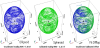
The main ellipsoid errors are the centroid vector offsets of -9, -2 and -2 nT; the scaling and orthogonality errors are negligible, as the raw data sphericity indicates, but their minor errors are also corrected for. The Figure 5c right panel arrow points out the translation of the raw blue ellipsoid toward the green corrected spheroid 0,0,0 origin, with the sphere on the centroid with corrected offsets, scaling and orthogonality. That the raw data ellipsoid is more spherical than ellipsoidal, with a calibration r.m.s. of 7.38 nT, indicates that the FVM after warm up is low noise to begin with, without calibration corrections. After calibration corrections though, the r.m.s. is lowered to 2.16 nT, which is a noise level improvement ratio (IR) of 3.4.
The landfill calibration profiles for the three survey days are seen in Figure 6, this image was previously presented and modified slightly from [1-3], with some of the following discussion presented in [3] also. Panels 6a, 6b and 6c are ground survey days 1 and 2 and UAV day 3 respectively. Statistics for the three days' profiles are seen in the Figure 6d table, with the yellow-highlighted bottom row the UAV day with some minor quality control (QC) de-spiking, as pointed out by the arrows in panel 6c. The Figure 6d table’s UAV day calibration r.m.s. statistics, seen in row 3, were used above for Figure 5.
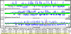
The 20 Hz low pass filter is used as the 200 Hz sampled FVM data is directly compared with the 20 Hz sampling AVM in a following gridded data comparison section. Beside FVM calibration statistics the data columns contain the landfill AVM mean base station and published Boulder, Colorado IAGA observatory mean TMIs during calibration. The AVM base and Boulder observatory TMI are measures of FVM reading stability over the three days. FVM ground day 1 has the largest offset from the AVM and Boulder readings, about 5 nT; and this offset is removed by leveling the FVM reading mean to the AVM base mean for that day. The AVM conditions the FVM data, a magnetometer role reversal. Past calibration practice has used an FVM to correct and compensate AVM data, here the fT resolution AVM base station corrects the FVM data for diurnals and base level offsets.
Figure 6d shows the raw TMI r.m.s. for the three days at 7.45 nT or below, calibration further lowers the r.m.s. into the 2.16 to 3.00 nT range, and the low pass further reduces these numbers into the 0.82 to 1.69 nT range. The higher r.m.s. for the UAV day may reflect more aggressive calibration motions causing a few obvious profile spikes. Removing the few obvious spikes from the TMI lowers the noise statistics highlighted in yellow on the bottom row. The resulting 1.81 and 1.20 nT r.m.s. after spike removal is thought to reflect residual magnetic gradient and active geomagnetic background noise superimposed on the system white noise. The corrected TMI low pass r.m.s. numbers, including the UAV day’s spiky 1.69 nT are all below 2.0 nT. This low-pass r.m.s. number, along with the UAV day unfiltered calibration-corrected 1.81 nT, and the 20 Hz filtered 1.20 nT r.m.s., can be compared with the Geological Survey of Canada (GSC) guideline helicopter FOM specification [21]. Though a groundbased calibration, these r.m.s. should be valid noise measures for an effectively omnidirectional isolated slung sensor subject to negligible platform noise. Any airborne slung sensor motion noise can be treated like any scalar slung sensor survey, using frequency filtering for removal if necessary.
6. Results and Discussion
The following discussion and images were presented in modified or modified form in [1-3], with additional discussion presented in the following two gridded TMI sections.
6.1 Comparison of ground and UAV FVM gridded TMI images
Figure 7 compares the FVM ground survey, this survey UCF 1 m, and the FVM UAV survey results in gridded TMI data format in (7a), (7b) and (7c) respectively. The UCF 1 m image approximates the UAV image, flown at an average 3 m height, which it does with its TMI range of 4221 nT being 2 nT off the UAV range of 4219 nT. The black arrows on the SE of the three upper images point out a dipole signature common to the three. It’s seen the UAV dipole response in 7c is attenuated; this attenuation is due to a few higher flight lines on the grid SE where the sensor was an average 5 to 6 m height above ground.
The two lower panel images 7d and 7e show the UAV data DCF 1 and 2 m respectively, with the TMI statistics for the five gridspresented in the table seen in 7f. The two DCF images, in effect, locate the UAV sensor height near or below the 2 m ground sensor, to approximate the ground survey TMI. It’s also used to reduce the signal attenuation seen for some higher flight lines as mentioned for the dipole seen in 7c. The Figure 7f table statistics show that the DCF 1 and 2 TMI ranges of 5077 and 5246 nT respectively, reasonably approximate the FVM ground TMI range of 5099 nT. The DCF 2 image is also convolution filtered to remove some minor high frequency noise exacerbated by the DCF; whereas the DCF 1 image was not. The black arrows on the SE of the two DCF images point out the same dipole signature seen in the upper three images. Both DCF filtered grids better approximate the overall survey ground FVM grid response and the local SE dipole seen in 7a, than does the unfiltered UAV image in 7c.
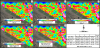
Though the two DCF grids are similar and higher resolution than the unfiltered UAV TMI, it’s also seen that the ground survey retains some higher resolution; likely due to an estimated 10 times slower walking speed of 0.4 m/s versus the 4.0 m/s airborne speed. Subsequently, the ground survey sensor 200 Hz readings return an approximate 10 times higher sample density. Also, as the ground sensor is maintained at a constant 2 m height, whereas the UAV sensor is slung and subject to minor sensor movement at the visually estimated 3 – 4 m sensor height; the ground survey data is consistently level on 2 m and without sensor height- related signal attenuation. This is best shown by the 7b image; the consistent 2 m ground survey sensor height produces a consistent UCF 1 image that produces a consistent approximation of a UAV survey 3 m sensor height, including a higher resolution dipole signature as pointed out by the arrow on the SE of the image. Conversely, the UAV survey has a few flight lines with a 5 to 6 m high sensor that attenuates the TMI signal on some lines, as pointed out clearly by the arrow at the dipole on the SE of the UAV survey grid seen in Figure 7c.
7. Comparison of FVM and Ground AVM Gridded TMI Images
Figure 8 compares the AVM ground survey TMI benchmark image (8a) with the FVM surveys’ ground (8b) and UAV DCF 1m (8c) gridded datasets. The FVM - AVM ground survey difference grid is seen in 8d, with the FVM ground - UAV DCF 1 m difference grid in 8e, with the TMI statistics for the 5 grids seen in the 8f table.
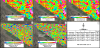
The AVM and FVM ground surveys were walked on the same 10 m spaced traverse lines at the same 2 m sensor height. Visually, the mapped signatures in 8a and 8b closely approximate each other. The difference grid in 8d reflects this, showing a random pattern, with no obvious line effects in either dataset. This is expected, as both the FVM and AVM tested have negligible heading effects. The random difference grid pattern has a zero mean as the FVM is leveled using heading effects. The random difference grid pattern has a zero mean as the FVM is leveled using a second AVM base station for diurnal corrections. The random difference signature pattern with an r.m.s. of 180.37 nT is likely due to ground surveyor off-line traverse wander of a few meters within each survey and between the two surveys, over the hummocky ground surface. A second source of random offsets is GNSS X and Y coordinate positional errors between the two surveys, as the standard GNSS used by both magnetometers have, at best, a positional accuracy of 2 to 3 meters, and the surveys were done on different days. It took two days to complete each ground survey, four days of traversing in total. That the FVM ground survey has a 600 nT broader range, is thought to be the result of the FVM traversing over a few positive and negative (+/-) peak signature amplitudes that the AVM traverses may have missed, and is not thought to be due to differences in FVM or AVM dynamic measurement ranges, resolutions, sensitivities or accuracies.
The FVM ground – UAV DCF 1 m difference grid has a mean value of +56 nT, with the ground FVM having the higher mean, this may reflect inverse distance signal attenuation between the 2 m high ground sensor with the slung UAV sensor height, at an average 3 to 4 m above ground. The 22 nT range difference between the two grids, 5099 nT for the ground and 5077 nT for the UAV DCF 1 m, indicates that the UAV DCF image is a reasonably close approximation of a 2 m high sensor ground survey. The ground - UAV DCF survey difference grid shows two subtle line effects, due to UAV flight height offsets, that appear related to battery swap lines. These line effects are not obvious in the UAV DCF grid. Aside from the subtle line effects and signature attenuation for a few high flight lines, this difference image has random signatures, showing that the UAV survey also, is not much affected by line heading effects.
8. Conclusions
A ground calibrated FVM sensor effectively becomes an omnidirectional scalar TMI magnetometer with a r.m.s. error attached to it, for both ground and UAV slung sensor surveys. Low pass filtering of 200 Hz sampled FVM TMI is effective removing 60 Hz noise in an urban environment, without a loss of data resolution.
The FVM UAV survey shows minor magnetic signal attenuation effects, being flown an average 1 to 2 meters higher than the ground sensor surveys, as expected. The gridded data attenuation is slightly exacerbated on a few higher flight lines, that in part appear related to battery swaps, as shown on the ground FVM – UAV FVM difference grid. The UAV flies back into the survey lines high initially, on the repeat lines, then settles down into a lower height after flying for one or two lines.
The ground FVM survey is a close approximation of the ground AVM survey benchmark. The UAV FVM data remains high resolution and low noise, with its DCF filtered products being reasonable approximations of the FVM ground data, where they could be considered for first pass landfill reconnaissance. A DCF UAV survey could be followed up with AVM ground survey real-time-display profiling over signatures of interest, for accurate ground staking and follow-up investigation.
While landfill surveying, ground and UAV scalar calibrated FVM did not require special sensor alignment, had no data drop outs, dead zones, returned no obvious heading effects, and required no line leveling prior to DCF filtering, and has a high gradient tolerance near ferrous surface objects like gas valves and steel fences.
UAV with RTK GNSS should improve survey flight height consistency, and active real-time Lidar or Radar may further improve vertical positioning, possibly sacrificing lighter UAV weight, battery life and times aloft, while increasing system and data processing complexity.
Competing Interests
The authors declare that they have no competing interests.
Acknowledgments
The author thanks the city of Golden, Colorado for permission to
walk the ground, and fly UAV magnetometer surveys over the landfill;
being able to undertake this study is much appreciated.
Note: Graphy Publications remains neutral with regard to jurisdictional
claims in published maps and institutional affiliations.