


1. Introduction
In agricultural farmland management and vadose zone research, knowledge of proximal soil physical properties within a couple of meters below the surface is important. In this zone, the subsurface soils are mostly unsaturated and their mechanical properties (bulk density, bulk and shear moduli, shear strength, and state of stress) and hydraulic properties (such as moisture content and water potential) are frequently influenced by agricultural activities (causing compaction), rainfall and seasonal events, and natural soil processes. It is desirable to develop a non-invasive technique that can measure and monitor the temporal and spatial variations of soil properties in situ.
For proximal soil sensing, a high-frequency multi-channel analysis of surface waves (HF-MASW) method has been developed [1-4], which measures soil shear wave velocity profiles from a few centimeters to several meters below the surface. The method is a modification of the conventional MASW method [5-10]. The MASW method is a seismic/acoustic technique based on spectral analysis of one type of seismic surface waves, Rayleigh waves, to determine the shear (S) wave velocity profile, i.e. the S wave velocity as a function of depth. The MASW method has been increasingly applied to geotechnical and civil engineering projects, such as mapping bedrock [11], detecting voids [5,12] and buried objects [13], determining Poisson’s ratio [14] and quality factor [15], evaluating the stiffness of water bottom sediments [16], delineating fault zone and dipping bedrock strata [17], and evaluating levees [18]. These MASW tests explore subsurface properties at depths from several meters to tens of meters due to the low frequency sources employed and the civil and geotechnical engineering targeted objectives. Consequently, the detailed soil properties of the upper few meters of soil cannot be accurately determined [7]. In contrast, it is in this shallow zone of soil that the HF-MASW method can effectively be applied. Using highfrequency excitations (up to a few kHz), the HF-MASW method can measure soil shear wave velocities of this very shallow soil zone, thus filling the gap of the conventional MASW method. Fundamentally, the S-wave velocity is related to soil mechanical and hydraulic properties. It is well known that the shear wave velocity is closely related to shear modulus, an important soil mechanical engineering parameter [19]. The shear wave velocity is controlled by the principle of effective stress [19-21]. As shown later, the effective stress is equal to the difference between total stress and water potential for unsaturated soil. Therefore, the measured S-wave velocity profile can reflect the temporal and spatial variations of soils due to rainfall events and water infiltration processes, to the existence of hard soil layers such as plow pans and fragipan (a naturally occurring dense soil layer), and to anthropologic activities (compactions).
The objective of this paper is to provide a review of the past works in the development and application of the HF-MASW method for proximal soil sensing. The physical mechanisms that relate the acoustic velocity to soil mechanical and hydraulic properties are first introduced. In the next section, practical techniques to enhance the HF-MASW method are presented. The HF-MASW experimental setup and procedure are described later. In the following section, several applications are reported including (1) measurement of soil profiles at test sites with different soil textures [4], (2) study weather and seasonal effects on shallow surface soils in a long-term survey [1], (3) monitoring soil profile variations during rain events [22], (4) detecting and imaging a soil fragipan layer [23], and (5) assessing compaction effects on farmland [24]. The discussion and conclusion are addressed in the final section.
2. Materials and Methods
2.1 Mechnaical and hydrological responses of the acoustic velocity of soils
Soils are heterogeneous assemblies of unconsolidated mineral or organic material, forming porous media and consisting of three phases: solid particles, water, and air. Their mechanical behaviors are determined by the discrete nature of the media, external and inter-particle forces, interconnected porosity, and multiphase conditions. On the other hand, acoustic waves traveling through soils interact with soil particles and interstitial fluids. As a result, the soil texture, structure, and hydraulic conditions affect acoustic responses, which, in turn, are sensitive to the variations of soil properties and conditions. Interested readers may refer to the references [19,25] for additional information about acoustics in porous media and soils.
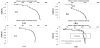
In a lab study, a tri-axial cell test was conducted to measure one of the acoustic velocities, i.e. longitudinal (P) wave velocity during the simulated soil compaction processes [20]. The resulting mechanical behaviors and acoustic responses of soils are displaced in Figure 1.
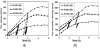
The curves in Figure 1(a) represent typical soil load-deformation behaviors of a remolded soil with three different confining pressures. The curves consist of the normal consolidation lines where the stress increases with strain, failure points where the maximum stresses are reached, and hysteretic behaviors, shown as steep loops. The corresponding acoustic velocities as a function of strain are shown in Figure 1(b). As one compares Figure 1(b) with Figure 1(a), the acoustic behaviors are very similar to those of the load-deformation curves. These similar variation trends between the stress vs strain curves and the acoustic velocity vs strain curves demonstrates that the acoustic velocity can be used as a promising parameter for measuring and evaluating soil mechanical properties and states of stresses.
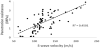
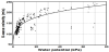
In a long-term survey, aiming at studying seasonal and weather effects on the acoustic velocity [21], the experimental results revealed the acoustic velocity’s responses to hydrological properties of soils in terms of water potential and moisture content, as displayed in Figure 2.
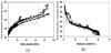
The data in Figure 2(a) demonstrates a general trend in which the acoustic velocity increases exponentially with water potential, while the acoustic velocities in Figure 2(b) decrease nonlinearly with moisture content. It is worth noting that water potential and moisture content are not independent but are inter-related through a moisture characteristic curve or water retention curve. The observations in Figure 2 indicate that the acoustic velocity is sensitive to the variations of soil hydraulic properties.
The above acoustic velocity responses to soil mechanical and hydraulic properties and conditions can be understood by using an empirical relationship between the acoustic velocity and the effective stress [19-21,25], as expressed by,
where V is the acoustic velocity which can be either the longitudinal wave (P-wave) velocity or the shear wave (S-wave) velocity, V0 is the corresponding velocity at 1kPa, the exponent β is an intrinsic soil property, and σ' is the effective stress.
The concept of the effective stress was first introduced by Terzaghi [26,27] in a form given by:
where σ denotes the external confinement force or the total stress applied to the medium, and μ the pore fluid pressure.
Terzaghi’s principle of the effective stress states that for a fully saturated soil, the soil fabric carries the stress difference between an external force and the pore water pressure. For unsaturated soils, Bishop and Blight [28] proposed a modified effective stress given by,
where μa is pore air pressure, μw is pore water pressure, and the quantity (μa-μw) is matric suction or the negative value of water potential, often measured by a tensiometer [21,29]. χ is a soil parameter that varies between 0 for dry soil and 1 for fully saturated soil-its value depends on the degree of saturation or matric suction [29].
The first term on the right-hand side of Equation (3) represents the component of net normal stress applied to the soil solid frame, which often contributes to soil mechanical behavior when it is subjected to external forces, such as compaction, or overburden pressure. The product term χ(μa-μw) represents the inter-particle stress due to suction, referred to as suction stress, which is related to soil hydrological properties in terms of water content, degree of saturation, and water potential [29].
The experimental evidence mentioned above and theoretical knowledge as formulated in Equation (1) through Equation (3) provide a substantial basis that acoustic velocity can be used as an effective parameter for charactering soil’s mechanical and hydrological properties. In proximal soil sensing, a non-invasive and in-situ technique is always preferred. For this purpose, the HFMASW method has been developed.
2.2 The enhanced HF-MASW method
When exploiting higher frequencies, the HF-MASW method is technically challenged by the fact that the attenuation of Rayleigh waves increases with frequency and distance [2] and the seismic energies of a vibration source decrease significantly at higher frequencies. In order to enhance the HF- MASW method, practical techniques both in the data acquisition and signal processing have been developed [2,3]. These techniques are (1) the self-adaptive MASW method using a variable sensor spacing configuration, (2) the phase-only processing algorithm, and (3) a nonlinear acoustic technique with gapped frequency band excitations, respectively. These techniques can effectively enhance the dispersion patterns and extend the measureable frequency range.
2.2.1 The self-adaptive HF-MASW method with a variable sensor spacing configuration
The self-adaptive HF-MASW method with a variable sensor spacing configuration has been described in detail in the literatures [2-4]. The concept of the technique is summarized below.
For a traditional and full spread length MASW method, a so-called overtone image, i.e. an intensity graphic representation in phase velocity and frequency space, is obtained by a 2-D wave field transformation method proposed by Park et al. [6] and its summation form is expressed as follows:
where f and c are frequency and phase velocity, E(f, c) the energy at the coordinates of (f, c) in phase velocity ~ frequency space, Rj(f, xj) the magnitude term of the fast-Fourier-transform of the jth time trace at offset xj, phase ∅j=2πfxj/c, N the number of the time traces, and denotes the imaginary unit. In this formulation, summation is made over the entire set of time traces and the Fourier transform Rj(f,xj) is usually normalized to unit amplitude for each trace.
For a self-adaptive MASW method [2-4], the near offset xnear (the distance between a seismic source and the first selected sensor), spreadlength L (the length covered by the selected subset of sensors), and the far offset xfar (the distance between a seismic source and the final selected sensor) are determined by the wavelength λ at each frequency:
The 2D wave field transformation is performed by summing over the time traces that satisfy Equation (5) and can be expressed as [31,32]:
where nnear and nfar are indices of the time traces that match closely the near offsets xnear and far offset xfar respectively. The term of (nfar–nnear+1) in Equation (6) is used for normalization. The outcomes of Equation (4) and Equation (6) are intensity graphs in phase velocity and frequency space, a so-called overtone image. In the overtone image, the dispersion curve, i.e. the phase velocity vs frequency can be determined from their dispersion patterns.
In order to overcome spatial aliases at higher frequencies and reduce the number of sensors, a variable sensor spacing configuration is applied, which features a progressively increased sensor spacing configuration. In practice, two sensor spacing configurations are often used, which combine an equal spacing configuration with a variable spacing configuration, in an attempt to best match the dispersion curve that tends to level off at high frequencies [2,4]. For example, a typical geophone array consists of 10 geophones with 2 cm equal spacing and 20 geophones with 2 cm incremental spacing and features a spread length of 4.4 meters.
2.2.2 The phase-only processing
For the phase-only processing, the magnitude term Rj(f, xj) in Equation (4) and Equation (6) is simply set to 1 and only the phase term is taken into the waveform transformation. From the wave propagation point of view, the phase term is related to time delay and is a property of phase velocity, whereas the magnitude term is determined by the intrinsic attenuation and geometric spreading and varies with frequency and distance. It has been proven that the influence of the frequency and distance dependent attenuation on the dispersion curve can be effectively eliminated by setting a constant magnitude, as long as the phase spectrum is reliably measured [3,32].
2.2.3 The nonlinear acoustic technique
In a HF-MASW test, a shaker is used as a controllable seismic source operating in a frequency sweeping (chirp) mode. The seismic excitation usually consists of three frequency bands to provide sufficient seismic energy with a tradeoff between sampling frequency and excitation duration. Initially three overlapped frequency bands were employed, representing low frequency (LF), middle frequency (MF), and high frequency (HF) bands, respectively. It was later found that the dispersion curves can be determined at significantly higher frequencies than their source frequency bands. It is speculated that due to the nonlinearities of soils, a so-called mesoscopic hysteretic elasticity [33-35], and of the vibration source through contact nonlinear mechanisms, higher harmonics could be generated, which extends the measureable frequency range of the dispersion curves. Taking advantage of this nonlinear phenomenon, the seismic excitation can now be divided into three gapped frequency bands. Doing so can increase the seismic energy coupling into the ground by maintaining the same chirp duration. For a given duration, narrowing the frequency range increases the number of cycles of chirp signals. This enhances the energy of the lower frequency components, especially for the LF band.
2.3 Experimental setup and the HF-MASW procedure
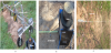
The experimental setup for the HF-MASW method consists of a seismic shaker and multiple vibration sensor placements along a straight line. Two seismic vibration shakers were used in the past. One is an electrodynamic shaker (Vibration Test System, Model VG-100- 6). The shaker weighs 30.4 kg with a size of 29.2 cm×26.0 cm×21.6 cm and provides 49.9 kg of peak force and a working frequency range from DC to 6500 Hz. A 11.3 kg copper cylinder is screwed on the top of the shaker to enhance energy transferring into the ground. The second shaker is a home theater actuator (TES-100 Actuator, 1-600 Hz, Crowson Technology) and weighs 1.6 kg with a size of 14.5 cm ×12.2 cm ×2.8 cm. The actuator can support maximum load of 453.6 kg. In operation, two 9.1 kg lead bricks are stacked on the top of the actuator to enhance the vibration force. A rubber sheet is placed between the actuator and the lead bricks as a cushion. Three seismic vibration sensors have been used (see Figure 3): a moving laser Doppler vibrometer (LDV, Polytec PI, Inc., Model PDV 100, DC-22 kHz) driven by a stepper motor used as a non-contact sensor to detect vertical particle velocity [1], an accelerometer (PCB Piezotronics, Model 352B, 2 Hz to 10,000 Hz) with multiple steps of insertions to measure surface acceleration [2-4,24], and a geophone array with 40 geophones (40 Hz, GS-20DM, Geospace Technologies) to measure surface vibration velocities [22].
Comparisons of the HF-MASW test performances among employments of the two shakers and three types of sensors yielded essentially identical results in resolving the dispersion curve at the frequency range investigated. The signals from the geophones can be simultaneously sampled by a data acquisition board (NI USB-6255, National Instrument) without any signal conditioning. Therefore, a HF-MASW system consisting of the actuator and the geophone array is recommended due to the reduced costs of equipment. The data acquisition board also serves for generating chirp signals. The chirp signals are amplified by an audio power amplifier (Stewart World 600, Stewart Audio Inc.) and fed into the shaker.
A HF-MASW test procedure includes four stages: (1) data acquisition, using the above mentioned shaker and sensors to measure multiple surface vibrations along a straight line (see Figure 3); (2) processing the detected signals, using the self-adaptive and phase-only techniques to obtain the overtone images, i.e., an intensity representation in phase velocity and frequency space (see Figure 4); (3) extracting the dispersion curves, i.e., the phase velocity as a function of frequency, from the overtone images; and (4) determining the soil profile, i.e., the shear wave velocity as a function of depth, by an inversion process (see Figure 5). The details of these procedures can be found in the literature [9].
A program written in LabVIEW (National Instruments, Inc.) is used to communicate between a computer and instruments for chirp signal generation, data acquisition, 2-D wave field transformation, and dispersion curve determination. A software package, SurfWave Academic (version 1.26a, H&H Geophysical LLC) is used for the inversion process.
3. Results
3.1 Soil profile measurements
The HF-MASW tests were conducted at four testing sites [4] using a single accelerometer inserting at different locations along a straight line (see Figure 3(b)). The first two sites (loess and coastal plain) were located at the Mississippi Agriculture and Forestry Experiment Station (MAFES) at Holly Springs, Mississippi. The loess soil is mapped as Providence silt loam (fine-silty, mixed, active, thermic Oxyaquic Fragiudalf). The second MAFES site is a Cahaba sandy loam (fineloamy, siliceous, semi-active, thermic Typic Hapludult). The soil at the third site was a Harleston sandy loam (coarse loamy, siliceous, semiactive, thermic Aquic Paleudult), at Pascagoula Beach, MS. The forth site was located at the Pontotoc Ridge-Flatwoods Branch Experiment Station of MAFES facility near Pontotoc, MS, which is an Adaton silt loam (Fine-silty, mixed, thermic Typic Ochraqualfs). This test site was used for a compaction study and treated by deep tillage using a subsoil shank. The site was kept undisturbed for several months, then the deep-tilled Adaton site was compacted using a John Deere 7320 tractor. The HF-MASW tests were conducted on both non-compacted and compacted Adaton soils for comparison purpose. The soil profiles in terms of the shear wave velocity were plotted in Figure 5.
In Figure 5(a), the Providence silt loam soil at Holly Springs presents a normal soil profile, featuring a monotonously increasing shear wave velocity trend with depth. The exploration depth at this site reaches a maximum value of 2.5 meters. In Figure 5(b), the Cahaba sandy loam at another Holly Spring site behaves differently from the silt loam with overall lower shear velocities than those of the silt loam profile. The soil profile in Figure 5(b) demonstrates a hard layer around 10 cm to 20 cm, followed by gradually increased shear wave velocity with depth. The exploration depth in this site is 1.2 meters. In Figure 5(c), the Harleston beach sand in Pascagoula, MS exhibits an increasing variation in the shear wave velocity within the depth of 50 cm. Below 50 cm deep, the velocity remains constant and then even slightly declines. This is due to the fact that the testing site is close to the shoreline where the soil is saturated below a shallow water table. In Figure 5(d), the non-compacted and deep-tilled Adaton soil at Pontotoc site presents low values of the shear wave velocities on the top 20 cm layer, reflecting the loose soil structure due to deep-tillage. Below 20 cm, the shear wave velocity increases slowly with depth. The compacted Adaton soil has higher shear wave velocity on the top soil than those of non-compacted soil, showing the compaction effects from wheel-traffic that consolidates the soil and raises the shear wave velocity [20]. The compaction effects are evident on the top 20 cm soil and can affect soil properties down to 60 cm deep.
In order to validate the HF-MASW tests, soil penetration tests were conducted at the testing sites using a penetrologger (Eijkelkamp, Agrisearch Equipment, Giesbeek, Netherlands). This device measures penetration resistance with a maximum depth down to 80 cm with 1 cm resolution. The plot of the S-wave velocity vs. the penetration resistance of these soils is shown in Figure 6, which yields a moderate linear relationship with the correlation coefficient r2 of 0.45. More details of the comparisons and discussions between the results of the HF-MASW tests and the penetration tests can be found in the literature [4].
In general, the penetration tests are more sensitive to vertical variations because of their vertical resolution of 1 cm. They are point-measurements and, therefore, susceptible to local heterogeneities. On the other hand, the soil profiles from the HF-MASW method are the averaged soil properties at mid-point along the survey line. Therefore, the drastic vertical variations, such as adjacent layering information and local heterogeneities, will be smoothed. These facts may explain the moderate correlation observed in Figure 6. In addition, one should keep in mind that the S-wave velocity and penetration resistance are two different physical parameters with different governing mechanisms. In-depth study of their relationship is required in the future.
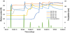
3.2 Long-term survey for weather and seasonal effects study
A long-term survey was conducted to study weather and seasonal effects on subsurface soil [1] with a moving LDV as a surface vibration sensor (see Figure 3(a)). The HF-MASW tests were conducted four times per day at irregular time intervals. The test was conducted on the University of Mississippi campus where the original soils of a thickness of about 10 feet were excavated and refilled with washed sand. This site can be regarded as a homogeneous medium without the presence of distinctive layers. During a one-year survey, the temporal variations of the soil temperature, water content, water potential, and P-wave velocity were monitored by the corresponding buried sensors, as plotted in Figure 7. Day 1 is Jan. 1, 2005. These sensors are thermocouples (Model TMTSS-125, Omega), time domain reflectometers (TDRs, Model 6005L2, Soil Moisture Equipment Corp.), tensiometers (Model 2710ARL06, 2710ARL12, Soil Moisture Equipment Corp.), and a pair of home-made acoustic probes, respectively.
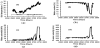
Several observations can be made from these figures. All the results show strong seasonal influence. The seasonal transition can be identified by the magnitudes and trends of these parameters. In general, the water content data indicates that the soil conditions were wet, moist, and dry in the winter, spring, and summer, respectively. The water potential and the P-wave velocity behave similarly, representing the phases of remaining low values in the winter, gradually increasing trends in the spring, and drastically soaring and falling trends in the summer. The similarity between the water potential and the P-wave velocity reveals a correlation between the two parameters as reported in the literature [21], confirming that soil suction stress is the predominant factor governing the effective stress for unsaturated soils. These figures also reveal weather effects due to precipitation. During each rainfall event, the water content, water potential, and P-wave velocity responded as initially abrupt changes followed by gradually recovering phases, reflecting the on-going processes of infiltration, drainage, and evaporation. In particular, the summer data show drastic variations due to extended droughts, heavy tropical storms, and intensive evaporation.
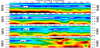
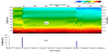
The temporal variations of soil profiles measured by the HFMASW method are shown in Figure 8, which reflects and matches the temporal changes of soil conditions due to weather and seasonal effects. Note that, since the HF-MASW tests were conducted on nonconsecutive days, the x-axis in Figure 8 is the time index number that represents the HF-MASW test numbers - not the time interval. In general, three different zones can be identified: the top dry, middle moist, and overburden pressure zones. The magnitude, extent, and depth of these zones, however, underwent gradual changes due to seasonal transitions and were intermittently interrupted by abrupt variations due to weather events. For example, the S-wave velocities in the top zone experienced an expected varying trend: maintaining relatively constant in the winter (Figure 8(a,b)), increasing slowly and consistently in the spring (Figure 8(c)), and soaring or falling rapidly in the summer (Figure 8(d)). Also, this top dry zone became closer and closer to the surface as summer approached. The horizontal discontinuity of the S-wave velocity in the zone is believed to be due to rainfall precipitation that had altered the soil conditions suddenly. The same observation and analysis can also be made to interpret the data in the moist zone. It is remarkable and anticipated that the most significant changes in the soil profile image occurred during the summer as shown in Figure 8(d). The dramatic changes in magnitude, extent, and depth happened not only in the top zone but in the moist zone as well, indicating an expanded influence of the weather that penetrated into deeper soils and turned the moist zone into a secondary dry zone. Similar variations can also be observed in Figure 8(c), where increased velocity regions can be found in the moist zone. In Figure 8(d) another interesting phenomenon can be found. Following weeks of extended dryness, heavy thunder storms brought top soils back into a moist condition. As a result, the values of the S-wave velocity in the top layer decreased to their low levels. Underneath the top layer, S-wave velocities remained high, indicating dry soil conditions. This high velocity zone may be explained by pre-existing dry soil condition, high rate of evaporation, and the insufficiency of precipitation to infiltrate deeper soils. These observations can be understood and interpreted with the concept of the effective stress, governed by soil suction stress/water potential for surficial unsaturated soils and by overburden pressure for deeper layers of soils [20,21].
The extracted S-wave velocities from the HF-MASW tests were compared with those of water potential at the same depth and time, as plotted in Figure 9. The data in Figure 9 falls into one curve that can be expressed as a power law relationship between the two parameters: Vs=a*Ψb, where Vs and Ψ are the S-wave velocity and water potential respectively. The curve fitting yielded the adjustable parameters: a= 96.0, b= 0.20, and a correlation coefficient r2 of 0.64. The scattering points in Figure 9 may be due to the hysteresis characteristic of soils. Similar power law relations between P-wave velocity and water potential have been reported [21]. This observation further confimes that water potential is the gorvening factor for the acoutsic velocity for unsaturated soils.
3.3 Short-term monitoring soil profile variations during rain events
The enhanced HF-MASW method used to investigate instantaneous variations of soil profile during rainfall events has been reported in the literature [22]. Recently, this experiment was repeated with newly installed TDR sensors and increased testing rate. The testing site was located on the campus of the University of Mississippi, near the NCPA building - the same testing site used for the study of seasonal and weather effects on soil profiles in 2011-2012. A geophone array with a variable spacing configuration was deployed in this test (see Figure 3(c)). The geophone array consisted of 40 geophones (40 Hz, GS-20DM, Geospace Technologies) with two combined spacing configurations: 10 geophones of 2 cm equal spacing plus 30 geophones of 1 cm incremental spacing that covered a total spread-length of 4.6 meters. A rain gauge was installed to measure precipitation. Five TDR sensors were buried at depths of 20 cm, 35 cm, 50 cm, 65 cm, and 80 cm, respectively, to measure soil moisture content. The HF-MASW tests, moisture content measurements, and precipitation recording were conducted continuously before, during, and after rainfall events with a sampling rate of one data set per 5 min.
Figure 10 shows the overall moisture content and precipitation. It can be seen from Figure 10 that the moisture content for the shallow soil changes rapidly in response to each rainfall event whereas the deeper soils react more slowly, reflecting the on-going water infiltration processes.
For the HF-MASW tests, two case studies were selected, which represent two different initial soil conditions and precipitations. The two cases were (1) initial dry soil with heavy precipitation and (2) initial wet soil with medium precipitation.
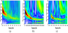
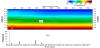
In case 1, the corresponding soil profile image and precipitation are displayed in Figure 11, which demonstrates the temporalvariations of soil profile in response to the rainfall and aftermath. Soil profile images up to 1.8 meters below the surface were obtained. Figure 11(a) shows the influence of rainfall on the soil profiles. As expected, the rainfall mostly affects the top soils, and this influence decreases with depth. For this case, rainfall infiltration depth can reach about 1 meter deep. From Figure 11(a) one also observes the gradual recovery stage after rainfall, manifesting a slowly increasing S-velocity with time. It is believed that this recovery stage is due to processes of evaporation, infiltration, and water redistribution. The transitions from dry, to moist, and to wet soil conditions are evident, and coincide with the rainfall events shown in Figure 11(b).
For case 2, there was a rain event one day before the HF-MASW test and therefore the initial soil condition was wet. This soil condition can be verified by examining the early stage of soil profile image in Figure 12(a). As compared with Figure 12(a) and Figure 12(b), every rainfall causes visible variations in soil profiles, manifesting in drops of S-wave velocity, followed by a recovery stage. However, the dynamic range of variations in the S-wave velocity are relatively smaller than those of the case 1. This is due to the initial wet soil conditions. One may refer to Figure 2 to understand the influence of initial soil conditions on the variation of the acoustic velocity. As seen in Figure 2, the acoustic velocity changes more drastically for dry soil than for wet soil per unit change in moisture content, indicating that adding more water to wet soil only leads to small decreases in the acoustic velocity.
3.4 Fragipan layer detection and imaging
A fragipan is a naturally occurring dense soil layer with very low organic matter, high bulk density and mechanical strength, and hard consistence when dry, but brittle when moist. It is restrictive to root and water penetration. Fragipans play a critical role in hydraulic behavior, erosion, and land use [36]. In order to detect and image a fragipan layer, a field test was conducted on the North Mississippi Experiment Station at Holly Springs, MS using both a two-dimensional HF-MASW test and invasive penetration tests [23]. Figure 13 shows the spatial distributions of the penetration resistance image measured by the penetration tests and the S-wave velocity vertical cross-section image obtained by the HF-MASW method at the testing site.
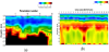
The image of Figure 13(a) represents a typical soil stratum formation in the vadose zone. Three distinctive layers can be identified. The topsoil from the surface to the depth of 0.1 m manifests a consistent high resistance layer indicating the existence of a hard top layer. This thin hardtop surface layer is often caused by rainfall impacts that form a surface curst. Moreover, at this location the surface was also compacted due to vehicle traffic. In addition, the surface was relatively dry in which case an increase in soil suction leads to an incremental increase in the effective stress [1,21] and hardens the soil. The middle layer around 0.1 m to 0.3 m exhibited declining penetration resistance, showing an opposite hydraulic effect on the soil stiffness, i.e. the increased water content softens the soil. The third layer, from the depths of 0.3 cm to 0.8 m, exhibited a gradually increasing trend in the penetration resistance with depth. This zone represents the transition from the argillic to fragipan layers. For most penetration points, non-penetrable zones are remarkably present at depths around 0.5 m deep as shown as black patches. It is believed that these nonpenetrable patches are the indication of the presence of fragic material in the argillic horizon that transitions with an irregular boundary into a fragipan. However, it is difficult to determine the thickness and extent of the fragipan layer from the penetration tests.
As in the case of penetration test, the S-wave velocity image in Figure 13(b) shows three distinct layers as characterized by their S-wave velocity: a top dry rigid layer, a middle moist soft layer, and a layer featured as monotonically increasing S-wave velocity with depth, at the depths of 0.1-0.3 m, 0.3-0.5 m, and below 0.5 m, respectively. The formation of these S-wave velocity layers can be explained by using the concept of the effective stress [26-28] and its power law relation with acoustic velocity [19-21,25]. In addition to the three layers, a high velocity layer (HVL) is apparent in Figure 13(b) at the depth around 0.8 m. The HVL stretches across the entire horizon with varying depths from 0.6 to 1.2 m. In order to compare with the results of the penetration test and the MASW method, a horizontal dashed line at depth of 0.8 m delineating the bottom line of the penetration test was drawn in Fig. 13(b) to facilitate the comparison. The comparison between Figure 13(a) and Figure 13(b) reveals that the spatial distributions, in terms of depth, size, and shape, of these high velocity zones are comparable to those of penetration test. Therefore, it is reasonable to regard these high velocity patches as the representations of the argillic-fragipan layers. Several observations can be made to further justify the identification of the presence of fragipan found in Figure 13(b). The HVL manifests distinctive contrasts among their adjacent soils, in accordance with the general fact that fragipans are usually characterized as high mechanical strength relative to overlying and underlying horizons, even when the upper layer is an argillic horizon [36], resulting in higher values in penetration resistance and S-wave velocity than those of surrounding materials. The irregular boundary, varying thickness, and horizontal– orientated formation of the HVL are in accord with the morphological characteristic of naturally formed subsurface structure of a fragipan. Further verification of the existence of a fragipan layer was confirmed by soil sample characterization and by digging a trench for visual inspection.
3.5 Farmland compaction study
Soil compaction induced by intensive use of agricultural machinery in farmland has adverse effects on crop growth and yield [37]. Compaction increases the bulk density and reduces the porosity of the soil. Increased mechanical impedance inhibits seed germination and hampers root growth [38]. Low porosity gives rise to insufficient aeration, reduction of water intake, and poor nutrient transport [39]. Heavy load decreases the permeability and capability of drainage and results in increased possibilities of surface runoff and erosion [40]. Compaction may deteriorate the self-remediation ability of soil and also affect the subsurface soils where a plow pan may develop [41]. An assessment of the influence of compaction on soil physical properties is necessary in agricultural research.
The testing site was located at the Pontotoc Ridge-Flatwoods Branch Experiment Station of MAFES facility near Pontotoc, MS, which is an Adaton silt loam (Fine-silty, mixed, thermic Typic Ochraqualfs) and characterized as a poorly-drained formed in loamy materials high in silt content with low permeability and a seasonally shallow water table. In order to remove effects of past tillage operations that could create a subsurface tillage hardpan, the test site was treated by deep tillage using a subsoil shank to break-up subsurface compacted layers. The site was kept undisturbed for several months following subsoiling. Then the deep-tilled Adaton site was compacted using a John Deere 7320 tractor.
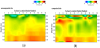
Two-dimensional HF-MASW surveys were conducted on both noncompacted and compacted sites [24]. As shown previously in Figure 5(d), examples of the soil profiles of non-compacted and compacted soils are presented, where the non-compacted soil presents low values of the shear wave velocities on the top 20 cm layer, reflecting the loose soil structure due to deep-tillage. Below 20 cm, the shear wave velocity increases slowly with depth. The compacted soil has higher shear wave velocity on the top soil than those of non-compacted soil, showing the compaction effects that consolidate the soil and raise the shear wave velocity [20]. The compaction effects are evident on the top 20 cm soil with an increment of above 20 m/s and can affect soil properties down to about 70 cm deep. From 40 cm to 70 cm deep, a hard zone with increased velocity occurred, as highlighted by a dotted rectangle in Figure 5(d). This high velocity zone is the consequence of compaction that creates a plowpan layer.
The cross-sections of the S-wave velocity images on both soils are shown in Figure 14. It can be seen from Figure 14(a) that the deep tilled soil presents low velocity at the top layer and the velocity monotonously increases with depth, featuring a normal soil profile. The compacted soil in Figure 14(b) exhibits an elevated velocity layer around 20 cm deep and at some deep locations the S-wave images show high-velocity patches around 50 cm, indicating a plowpan. Thus the influence of compaction on the soil properties can be assessed by the S-wave velocity image.
4. Discussion
Several practical concerns for conducting a HF-MASW test need to be addressed. The first concern is the factors that determine the exploration depth. In general, the deterministic factors could be the power delivered by the shaker to the ground, the lowest excitation frequency, and the spread length. In order to explore deeper soil profiles, more powerful shaker, lower beginning frequency, and longer spread length are required. However, the attainable penetration depth also depends on in-situ soil properties. The second concern is the measureable top layer depth, which is equal to the one third wavelengths at the highest resolvable frequency in a dispersion curve [42]. According to this rule, smaller sensor spacing and higher frequency excitation would be of benefit to obtain a higher frequency dispersion curve. In reality, it is not necessarily true. The surface soil condition also plays an essential role in determining the highest resolvable frequency. Under favorable surface wave propagation conditions, such as an intact, flat, and homogenous soil surface, the dispersion curve can be measured up to 2 kHz with 5 cm spacing [43]. In contrast, unfavorable soil conditions such as surface cracks, roughness, horizontal heterogeneity, and uneven moisture distributions in the form of moisture pockets would hamper the surface wave propagation due to scattering and attenuation effects and result in a dispersion curve with less resolved frequencies. The third concern is the disturbed soil condition. It is found that the HF-MASW tests conducted at freshly mechanical disturbed sites cannot generate reliable dispersion patterns at the frequency range that is equivalent to the corresponding depths of disturbance. It is speculated that the loose soil aggregates reflect and scatter surface wave energies. From our experience, it usually requires waiting several weeks or months to conduct a HF-MASW test after a mechanical soil disturbance. One may refer to the literature [4] for more detailed discussions.
A guideline for a sensor geometry configuration and data acquisition parameters was recommended in the literature [4], which is described as follows with minor modifications: the home theater actuator (TES-100 Actuator, 1-600 Hz, Crowson) and a geophone array (40 Hz, GS-20DM, Geospace Technologies) will be suitable as they reduce the cost of the equipment. The frequency ranges for the seismic excitations are 20-80 Hz, 200-500 Hz, and 600-1200 Hz with corresponding chirp durations of 10 s, 6 s, and 4 s for LF, MF, and HF bands, respectively. Very often, the HF band can be omitted if the top surface soil properties at depth of 10 cm are not of interest. Two geophone array configurations can be implemented. For a shallow soil profiling, a geophone array consists of 10 geophones of 2 cm equal spacing plus 30 geophones of 2 cm incremental spacing that covers a total spread length of about 4.6 meters. This geophone array will normally yield an exploration depth around 2 meters. For deeper soil depth, the geophone array configuration can be adjusted [4].
To validate the HF-MASW results, penetration tests were conducted as shown in Figure 13. The correlations among the S-wave velocity extracted from the HF-MASW tests, the penetration resistance, and the water potential were demonstrated in Figure 6 and Figure 9. Ongoing research will attempt to define the relationship among these parameters. Also, undisturbed soil sample characterization can be used for validation.
In general, the HF-MASW method is a seismic/acoustic technique. It noninvasively measures the shear wave velocity profile at a depth up to 2.5 meters. The method is unique because the S-wave velocity is related to soil mechanical (shear modulus, shear strength, bulk density) and hydraulic (moisture content and water potential) properties. However, due to the inherent nature of the surface wave method, the soil profiles derived from the HF-MASW method are the averaged soil properties at the mid-point along the survey line. Therefore, the drastic vertical variations, such as adjacent layering information and local heterogeneities, will be smoothed. Furthermore, the current HF-MASW method requires inserting sensors such as accelerometers and geophones into the ground at different locations. It is suitable for long-term monitoring and soil profile measurements at a specific location, like the applications presented in this paper. For large area surface mapping, it is prohibitively labor-intensive and time-consuming. It is desirable to build a mobile system, such as a high frequency land streamer, along with a multi-channel data acquisition system that can simultaneously sample multiple channels. Moreover, there is an ongoing research project aiming at developing a non-contact sensor array system. This multi-sensors system will exploit a so-called seismo-electric effect [44], i.e. a mechanism that seismic vibrations can locally generate electromagnetic signals. An electromagnetic sensor will be developed to detect the surface vibrations. Upon succeed; a series of this electromagnetic sensor will form an array to conduct HF-MASW in a non-contact manner.
5. Conclusions
This paper reviewed the developments and applications of the HF-MASW method for proximal soil sensing. Using this HF-MASW method, the spatial and temporal variations of soil properties, in terms of the S-wave velocity profiles, from a few centimeters to a few meters below the surface were measured. It has been demonstrated that the HF-MASW method can be applied for measuring soil profiles with different soil textures, monitoring weather and seasonal influences on soil, capturing instantaneous soil profile variations during rain events, detecting and imaging a fragipan layer, and studying compaction effects. Practical concerns and guidelines for conducting and validating the HF-MASW test were described, and the advantages and disadvantages of the HF-MASW method were summarized.
Competing Interests
The author declare that there is no competing interests regarding the publication of this article.
Acknowledgments
The author wishes to express his appreciations to Glenn V. Wilson, James M. Sabatier, Craig J. Hickey, and Mark W. Shankle, Alan Hudspeth, and Allen Gregory for many year’s collaborations, technical supports, and inspiring discussions.
Abbreviations