1. Introduction

Let us begin with the definition of a height system. Height system is a conglomerate of two things: a reference surface of heights equal to 0 (the height or vertical datum) and properly defined heights. These two entities must be treated and judged together as one entity.

What height systems are being used in practice?

Orthometric height system, which consists of the geoid as its datum and “orthometric heights”, H^O, measured along gravity plumb line. Gravity values are needed to convert the observed (levelled) heights to orthometric heights that then become “properly defined”. The geoid is referenced to the reference ellipsoid.

As a side issue we must mention here the Dynamic height system. “Dynamic heights”, H^D; they have no geometrical meaning but do have definite physical interpretation: points of the same dynamic height are guaranteed to lay on the same equipotential surface. In other words, any fluid is guaranteed to flow from a dynamically higher point to dynamically lower point. The datum of these heights is also

Normal height system consists of quasigeoid as a datum and “Normal heights”, H^N, measured along normal gravity plumb line. Gravity values are needed to convert observed height differences into normal height differences. More about these issues later.

How is a (practical) height system realized in practice? There are two issues here: realization of the datum, i.e., the “practical datum” and transformation of observed (levelled) heights to “proper heights” (in a transformation that makes use of real gravity values).

1. How is a datum for orthometric, dynamic and normal heights practically established? (Note that the geoid and quasigeoid are identical at sea which indeed includes the shoreline.)
2. How are properly behaving heights derived from observed height differences as obtained through the levelling process? Gravity values are needed.

Practical datum consists of one or more benchmarks whose heights are proclaimed to be known. For practical reasons, these benchmarks are usually located close to sea shore. An actual situation is shown in Figure 1 which portrays all the components of a typical setup involving a reference bench mark that represents (one of) a practical “datum point”. The main piece of hardware of such a setup is the tide gauge that registers temporal variations of the sea level supplying thus the data (time series) needed for the estimation of the height of the reference bench mark.

Figure 1: Typical setup of a reference bench mark representing one practical datum point [2].

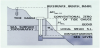
How is the local value of Sea Surface Topography (SST) obtained? By SST we understand a surface the sea attains after a very long time averaging. If the sea water were homogeneous and stationary, this surface would be a level surface, i.e., one of the equipotential surfaces of the gravity field and the SST would be everywhere identically equal to 0. Clearly, sea water is neither stationary nor homogeneous and SST thus varies from point to point within about ±1.5 meters and is also time dependent. It is the variable involved in establishing any height system which is most difficult to determine [1].

Turning now to the evaluation of proper heights, this evaluation consists of taking properly into account the effect of gravity. As we shall explain a little later, gravity plays the most important part in the definition of height, much as it plays the most important role in the definition of weight. It is gravity that will assure that the height difference between any two points will remain the same whichever way we chose to carry out the levelling between the two points; this property is known as holonomity and we shall again discuss it a bit later.

Both orthometric and dynamic heights refer to the geoid, one of the equipotential surfaces that follows somewhat closely the Mean Sea Level. The geoid, as a height datum, has to be anchored to the reference ellipsoid. Practical datum is the height of the reference bench mark(s) as determined by tide gauge(s) following the procedure described above when often enough the SST is not known and thus not considered. Then the difference of the theoretical and practical approaches is the already discussed SST.

Transformation of observed level differences to orthometric or dynamic height differences involves gravity. As said earlier, orthometric heights are geometrically meaningful but not physically meaningful - water may run up the “orthometric” hill. Dynamic heights, on the other hand, are physically meaningful but not geometrically meaningful.

Normal heights are referenced to a datum called quasigeoid, a computed artificial surface introduced by Molodenskij that runs within 2 meters on each side of the geoid. The quasigeoid also needs to be referred to the reference ellipsoid. Practical datum for normal is the same as for orthometric heights.

Transformation of observed level differences to normal height differences again involves gravity in a similar way as with orthometric heights as we shall see later. Normal heights are not physically meaningful but would be geometrically interpretable if it were not for the quasigeoid. Both orthometric and normal heights may be derived from potential numbers or dynamic heights, both the latter being physically meaningful.

Geodetic heights were never meant to serve as practical heights. They are not observable by terrestrial techniques. Their datum is the reference ellipsoid, hypothetical surface, adopted by convention. Geodetic heights h are computed from 3D satellite determined positions as accurately as implied by the accuracy of the 3D positions. They are measured along the normal to the ellipsoid and are sometimes incorrectly called “ellipsoidal heights”. No gravity is needed in their determination. But they are very important in measuring congruence of other height systems - see later - and in modern heighting.

The concept behind geodetic height determination is as follows: 3D Cartesian geocentric position determined from observations to GNSS satellites [3], i.e.,

( x y z ) (1)

gets transformed into the geodetic curvilinear coordinate system referred to a geocentric reference ellipsoid of revolution of major semi-axis a and eccentricity e. In this coordinate system, the 3D position reads:

λ= tan −1 ( y x ) h= x 2 + y 2 coscosφ −N φ= tan −1 z x 2 + y 2 ( 1− e 2 N N+h ) −1 (2)

Where, h is the sought geodetic height. N is the radius of curvature of the prime-vertical section. There exist various algorithms for computing h from the 3D Cartesian position [4] which we do not want to get into.

Figure 2: Relation between 3D Cartesian geocentric position and geodetic height.

2. Judging the Propriety of a Height System

The propriety of a height system should be judged according to the following three criteria: practicality, congruency, and holonomity.

2.2 Congruency

The height of the datum above the reference ellipsoid, either the geoidal height N or the height anomaly ζ, plus the respective height above the datum, either H^O or H^N , equal to the geodetic height h to at most third order error, i.e.:

H O +N =  H N +ζ= h (3)

(cf., Figure 3). It is important to mention that similar relation does not hold for dynamic heights. Equation (3) show geodetic heights have been used in practice up until recently. If we know h from GNSS, and have an accurate regional geoid we can determine orthometric heights from

Figure 3: Definition of congruency.

H O = h–N (4)

2.3 Holonomity

This property states that the integral of each differential, either dH^O, dH^D or dH^N, taken along a closed loop, must equal to 0:

∮ dH = 0 (5)

This is a necessary condition that enables us to adjust levelling networks. This property also ensures that the height difference between any two points of interest remains the same for whichever route we follow for the levelling, i.e., each point on the Earth surface has only one height associated with it [5,6].

What follows now is the theoretical argument that shows how observed (levelled) heights are to be transformed into proper heights, i.e., making them holonomic . A proper height H is defined differentially by:

g=−gradW→g=−∂W/∂H (6)

where g is the gravity vector and W represents the potential. Thus:

dH=− 1 g dW→δH=− 1 g δW (7)

where dH is a height differential and δH represents a height difference. This is how gravity g comes into the definition of height.

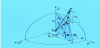
The situation is shown graphically in Figure 4. Even though point P'₁ should have a unique height with respect to the geoid, of potential W₀, its levelled height depends on the path, either starting from P₀ or from P₂, even though both starting points lie on the geoid (H = 0).

Figure 4: Illustration showing that observed heights are un-holonomic.

We should mention at this point that geodetic height sh, due to its geometric characteristic, can be considered holonomic. This property geodetic height possesses can be understood by rearranging Equation (3) to determine the geodetic height between two points (Δh= h₂ - h₁; ΔN =N₂–N₁; ΔH⁰ = H⁰₂ - H⁰₂):

Δh =Δ H O +ΔN⇒ h 2 = h 1 +Δ H O +ΔN (8)

What Equation (8) tells us is that independent on what path we choose to go from point 1 to point 2, the geodetic height h₂ is unique.

3. Why not Use the Geodetic Height System?

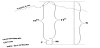
“Why not use the geodetic height system in practice?” This is a very often asked question that makes some sense as the ease with which we can measure and calculate geodetic heights h for almost any point on the surface of the Earth increases steadily. A typical Standard Deviation of a satellite determined height h is now about 3 cm, good enough for many applications. The main problem is its datum: in the geodetic height system the height of the sea shore varies between -100 m and +100 m which makes it difficult to work with in practice in a meaningful way [7]. Figure 5 shows why geodetic heights are not practical, useful for practice: the datum (h = 0) for geodetic heights crosses the Engineering building at the University of New Brunswick, located some 80 km from the sea. Who would be interested in working with heights referred to this datum?

Figure 5: why geodetic heights are not useful for practical work.

But as we have seen from Equation (4), we can obtain the orthometric height, H^O, from geodetic, h, when the geoidal height, N, above the reference ellipsoid is known. As stated above, geodetic height can be now determined to an accuracy of about 3 cm (standard deviation). If geoidal height N is known with adequate accuracy, which it is in places where good gravimetric data coverage is available, orthometric height can be determined to a comparable accuracy. This is the case with regional geoid models such as the UNB Stokes-Helmert geoid [8,9] that use both satellite and terrestrial data.

So, can we use one of those global satellite or combined models that can give us the geoidal height accurate to a few centimetres to compute orthometric height anywhere on the surface of the Earth? Not really! These global models may be quite good in some places, where there is an abundance of terrestrial gravity data, but quite bad in other places. Even in localities where global models work relatively well, the more accurate regional geoid should be preferred.

4. Why not Use the Molodenskij Normal Height System?

This system became quite popular in some European countries since about the 1980’s as it is easy to work with locally and regionally. Globally, its datum, the quasigeoid, is a fairly complex surface with folds, sharp edges and other “mathematically unfriendly” features, making it utterly inapplicable as a height datum. In practice, the quasigeoid is sometime obtained as a byproduct of the geoid computation by adding to the geoid an approximate correction.

Quasigeoid is defined in the following way: for each point (r_r,Ω) on the Earth surface there exists one and only one real potential value W(Ω). Draw a radius vector from the centre of the Earth to the point (r_r,Ω) - whose length is rt. Select the point ((r_r -ζ,Ω)on the radius vector at which the normal potential U(Ω) is numerically equal to the value of the real potential W(Ω) at the Earth surface. The value of ζ, called the height anomaly, positive or negative, constitutes a point on the telluroid, defining thus a new surface called telluroid. The negative height anomaly is, by definition, the height of the quasigeoid below or above the reference ellipsoid for the direction Ω (cf., Figure 7).

Simple! Yes, but what happens under a terrain overhang, where the radius of direction Ω intersects the surface of the Earth at 3 points and not 1 (cf., Figure 6)? As under overhangs there will be 3, 5, … values of ζ(Ω), the quasigeoid under the overhangs is not a mathematical function in the horizontal coordinate system (Ω). As it is not a function, it is not defined and it makes no sense to inquire if the quasigeoid is in these areas unique, finite, or anything else. How can we use a surface that is not defined in some areas as a reference surface for heights? Answer: the quasigeoid cannot be used as a global height datum, but it can be used locally or regionally in regions with smooth topography. And, of course, contrary to the belief held by some geodesists, discretization of the height system cannot be used to bypass the fatal problem of the quasigeoid not being defined globally.

Figure 6: shape of quasigeoid under a terrain overhang.

Figure 7: On the definition of Normal height.

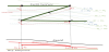
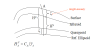
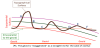
Figure 6 shows what the fold in the quasigeoid looks like. To estimate the values involved, let us make the following simple derivation. The size of a fold is given as the difference between two height anomalies ζ_A and ζ_B along the radial distance r_t as:

Δ ζ AB = ζ A − ζ B = ( W A –  U A )/γ− ( W B –  U B )/γ = ( W A –  W B )/γ− ( U A –  U B )/γ (9)

Now, considering that:

W A –  W B = − g ¯ AB Δ H AB (10)

and similarly:

U A –  U B =− γ ¯ AB Δ H AB (11)

Thus,

Δ ζ AB =(− g ¯ AB + γ ¯ AB )Δ H AB /γ=− δg ¯ AB γ Δ H AB (12)

where δg ¯ AB stands for mean gravity disturbance between points A and B.

To estimate the magnitude of the fold, let us assume the magnitude of δg ¯ AB to be 100 mGal and ΔH_AB as 1000 metres. For this combination, the magnitude of the fold Δζ_AB would be about 10 cm.Final verdict: the quasigeoidal fold may reach a few decimetres in either positive or negative direction. This clearly cannot be remedied by discretization or any other artificial means even if one wishes to disregard the problem of the failure of the quasigeoid being a mathematical function.

There are also other problems with the quasigeoid which is not a well behaved surface even in the areas where it actually is defined.

5. The Best System to Use

The only clear winner appears to be the classical system consisting of the accurate regional geoid and rigorous orthometric heights [10,11]. Some applications may require the use of dynamic heights but the datum for both orthometric and dynamic heights is the same: the geoid. Let us restate the reasons leading to this conclusion.

1. The datum, geoid, is a very smooth surface, convex everywhere, at sea as well as on the land, i.e., an ideal for a datum.
2. The zero-height surface (datum) approximates the average Mean Sea Level and this satisfies the usual practical requirements.
3. Both orthometric and dynamic heights are holonomic; consequently, orthometric and dynamic height networks can be easily adjusted.
4. Orthometric heights have a clear geometrical interpretation and dynamic heights have a clear physical interpretation.
5. Because the classical system is congruent, orthometric height can be also determined simply as a difference of geodetic and geoidal heights.
6. The datum can now be determined to an accuracy of better than 1 cm (standard deviation) in low lying areas and somewhat worse in higher altitudes.
7. Levelled height differences can be now converted to orthometric or dynamic height differences to a centimeter accuracy [12].
8. Dynamic height can be computed from orthometric height if gravity in the area is known.

6. Appendix: Systems of Height

Before the discussion that follows on Systems of Heights, it is useful to clarify the meaning of the terms “proper height”, “holonomic system” and “physically meaningful” heights.

Proper heights, or properly defined heights, are heights that take real gravity into account in their definition. They are holonomic, a property that assures they are uniquely defined.

The term physically meaningful height means that any fluid flows downhill. Only dynamic heights and geopotential numbers satisfy this definition.

Let us start with the Geopotential Numbers, the most natural height system. It uses the earth’s gravity potential W as “height” is unique (a point can lay on only one equipotential surface). Considering the difference between two close together equipotential surfaces as:

dW =−g dH (A.1)

We can define the geopotential number C of a point A from the geoid (indicated by the subscript 0) as:

C A =Δ C 0A = C A –  C 0 =  W 0 –  W A =−Δ W 0A = ∫ 0 A gdL ≈ ∑ k=0 A g ¯ k δ L k (A.2)

where L represents levelled height. The higher the point the smaller the potential, for A above the geoid W₀>W_A, thus the geopotential number grows with height.

Geopotential numbers have a somewhat cumbersome unit, length × acceleration. To have height expressed solely in units of length, the geopotential number is scaled by a reference gravity, resulting the Dynamic Heights:

H D A =  C A /G (A.3)

The reference gravity G is usually chosen as the normal gravity γ for a reference latitude φ_R. Points on same equipotential surface have the same H^D (as well as the C). H^D has definite physical meaning: water flows down the hill but it has no geometrical meaning because of the non-parallelism of the equipotential surfaces. Dynamic heights are unique and holonomic and equal to zero for points on the geoid.

Orthometric Heights are the closest geometric realization of dynamic heights. It is defined by scaling the geopotential number by an actual gravity value:

H A O = C A / g ¯ A (A.4)

where g ¯ A is an integral mean gravity between the geoid and point A. Because the actual value of g ¯ A is unknown, H^O can only be estimated. Points on same equipotential surface do not necessarily have the same HO. This characteristic breaks down the physical meaning of orthometric heights, as water may run up the “orthometric hill”. Nonetheless, it has a definite geometric meaning and is thus used extensively in technical practice. Orthometric heights are holonomic and, like dynamic heights, equal to zero for points on the geoid.

How are orthometric heights evaluated? As g ¯ A is an integral average of gravity between the geoid and the observation point A taken along the plumbline of point A, it cannot be determined accurately. Helmert proposed a model whereby gravity changes linearly with depth with a constant gradient of 0.0848 mGal/m (model known as Poincare- Pray’s gradient). The mean gravity is thus estimated as:

g ¯ A = g A +0.0424  H A O (A.5)

Approximate orthometric heights computed from this model are known as Helmert’s (approximate) orthometric heights. Helmert’s approximate heights may have errors of up to one decimeter level in mountainous regions.

Orthometric heights can be evaluated more rigorously by taking into account observed gravity and, possibly, variations in topographical density. There exist several techniques for improving the accuracy of orthometric heights. The latest, and most comprehensive, formulated at the University of New Brunswick, takes into account not only the observed gravity at the Earth surface but also the lateral variations of topographical mass density [10,11]. The accuracy of these more rigorous orthometric heights is now about one centimeter, i.e., better than the present accuracy of geodetic heights.

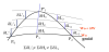
It is interesting at this point to provide a visual comparison between dynamic andorthometric heights, emphasizing the difference between physics and geometry. This is done with the help of Fig A.1. It shows 6 points on the Earth’s surface, contained by 3 distinct equipotential surfaces. It also shows the geoid, which is also an equipotential surface, represented as a straight line to enhance the impact of the example. Points on the same equipotential surface have the same dynamic height. This is the case of points A, E and F, points B and D, and point C. Points of same vertical distance from the geoid have the same orthometric height. This is the case of points C, D and F. The different effects of physics and geometry can be appreciated by looking at points E and F. Even though the orthometric height of point E is larger than the orthometric height of point F, water would not flow from E to F since both points lie on the same equipotential surface, i.e., E and F have the same dynamic height.

Figure A.1: Dynamic and orthometric heights.

Normal Heights are also proper heights. They are defined as:

H A N = C A γ ¯ A (A.6)

Where γ ¯ A is the mean normal gravity between the geoid and point A. Points on the same equipotential surface do not (generally) have the same normal heights. Normal heights have no physical meaning but a definite geometrical meaning. They are holonomic and equal to zero for points on the geoid.

Competing Interests

The authors declare that they have no competing interests.