1. Introduction

Unmixing hyperspectral signals and prole is still a challenge faces environmental, remote sensing, and geoscience communities. Hyperspectral data provide wealth of information about the physicochemical conditions of earth and extraterrestrial targets. However, the purity level of the spectra is a major challenge. Very often the hyperspectral proles contain several end members or components. In theory if a mixed spectra can be simulated using a mathematical approach then an inversion technique would reveal the end members. This approach was tested to simulate mixed spectra of different ratios of this binary system of Na₂SO₄-MgSO₄. On earth these chemicals salts of high enough concentrations can be considered economic minerals and salts that can be used in several industrial applications. For example, Na₂SO₄ is used in manufacturing wood pulp, glass industry, thermal storage, drying agent. Whereas magnisum sulfate is used commonly as epsom salt for medical purposes, and used in agriculture to increase sulfer or magnesium concentrations in soil, and it is used as brewing salt in beer among other uses. On Mars these salts have been investigated as an analogue to explorer the presence of microbes that possibly inhabit cold MgSO₄ rich brines in Mars. This binary system is also an adequate analogue of the martian salts and its salty regolith. For more details about the endmember extraction and unmixing, we refere to [8-14,18-21].

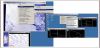
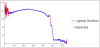
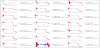
An example from spectral prole extracted from AVRIS image of White Sand in New Mexico, USA is shown in Figure 1. However, the data used in simulation here were obtained using the HR-1024i from the Spectra Vista Corp. (SVC) which is the latest model from their next generation of high performance single-beam eld spectroradiometer measuring over the visible to short-wave infrared wavelength range (350-2500nm).

Figure 1: Spectral proles matching as extracted from AVRIS image.

Reflectance spectroscopy and hyperspectral imaging analysis has picked up because it is reliable, fast, and less expensive and not intrusive [7]. However, spectral patterns for mixed materials can't be visually understood. Spectral pretreatment techniques must be applied to smooth spectral graph such as data normalization, continuum removal among other methods. We hypothesis that if the mixed spectra can be simulated mathematically, then we can obtain the end members that make up the mixed spectra. Toward this end, mathematical approaches or models that describe the reectance process in terms of several variables that control light reflection have been used extensively by Hapke in [6]; Pieters and Mustard in [1,15]; Robertson et al. in [16]; and Grumpe et al. in [5]. In the present study, we use wavelet approach to simulate and invert the mixed spectra. Wavelet methods are simple and computationally effective, and can be implemented in real-time. It is proven that wavelet reconstruction is an efficient way to represent functions, operators and big data set due to the capability of wavelet coecients to characterize image/signal discontinuities (i.e., noise) at different scales. In fact discrete wavelet transform (DWT) can be used in various applications, such as data simulation, image compression and coding. DWT refers to wavelet transforms for which the wavelets are discretely sampled. Wavelets provide a spatial frequency reconstruction, very useful in smoothing problems, in particular in density and regression approximation, having excellent statistical properties in data smoothing. They oer frequency and location time representation of data allowing adaptive ltering, estimation and smoothing. Two of the main advantages of wavelet representation is to provide an interpretation of the spectra and minerals related to the given data, using few number of high pass lters (coeffcients) and to provide a more concise representation because it minimizes the amount of redundancy in the coefficients and used to remove sparse noise from the signal.

Information of a hyperspectral image is heavily related to the shape of reectance spectra, which is recovered and represented in the magnitudes of its wavelet coefficients. The wavelet transform is an effective tool in many image processing applications due to the capability of wavelet coeffcients to characterize image/signal discontinuities (i.e., noise) at different scales. The DWT provides a more concise representation because it minimizes the amount of redundancy in the coefficients and used to remove sparse noise from the signal.

The simulation is done by performing three methods, Lagrange interpolation, and Daubechies and Haar wavelet threshold denoising methods, to simulate the given data. The original data can be recovered rst from Lagrange coffiecients and secondly by the (Daubechies and Haar) wavelets coffiecients through so called discrete threshold wavelet lter banks. In order to facilitate the simulation analysis and processing, and as a sample, we considered the reflectances of the wave lenght range 250-2500 nm of the binary system of Na₂SO₄-MgSO₄, then its Lagrange and wavelet threshold transform/interpolation should be discretized. The advantages of the interpolating curves using the methods above is that the entire data can be inferred as if we observe a dense enough set of points and only small amount of coffiecients are needed to achieve accurate approximation.

2. Metheodolgy

In this study, laboratory experiments under controlled conditions have been carried out to prepare pure Na₂SO₄ and MgSO₄ crusts and their mixtures. Analytical grade compounds of Na₂SO₄ and MgSO₄ were considered in this study. The salts were dissolved in water in 1000-ml volumetric asks. Total quantity of 200 ml of each solution were removed and placed in glass Petri dishes. The water was removed from the Petri dishes by evaporation at 40° C in an electric oven for 12 hours, then the samples were removed from the oven. Immediately following the removal from the oven, the samples were placed in a desicator, after which the reectance readings were made. A HR-1024i spectroradiometer was used to obtain the reflectance readings. Most of salts encountered in soils are a mixture of two or more type of salts. Sets of chemically mixed salt samples were prepared from which the pure salts were made using the same steps as described above. The mixing proportions are in 1 : 0, 0:75 : 0:25, 0:5 : 0:5, 0:25 : 0:75, and 0 : 1 weight mixing ratios. The spectra of the mixed samples were compared with the spectra of the pure samples solution fraction. All the pure and mixed samples were examined under petrographic and binocular microscopes for crystal size and morphology observations. Another runs were done by placing soil in the Petri dishes allowing the salt crus to grow on the top. In the ternary system consisting of sodium sulfate and magnesium sulfate, the following solid phases appear in the temperature range from -10° to 110° C:

1. Ice
2. Na₂SO₄∙10H₂O, glauber's salt
3. Na₂SO₄, thenardite
4. MgSO₄∙12H₂O, magnesium sulfate dodecahydrate
5. MgSO₄∙7H₂O, epsom salt
6. MgSO₄∙6H₂O, hexahydrite
7. MgSO₄∙H₂O, kieserite
8. Na₂SO₄∙MgSO₄∙4H₂O, bloedite
9. Na₂SO₄∙MgSO₄∙2.5H₂O, löweite
10. Na₂SO₄∙MgSO₄, vanthoffite

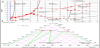
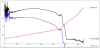
The temperatures and concentration ranges at which these solids appear are shown in the Figure 2. The phase diagrams shown on these pages are calculated with the Extended UNIQUAC thermodynamic model (http://www.phasediagram.dk/default.htm). The equilibrium lines and the experimental data in the diagram represent compositions and temperatures at which two solid phases are in equilibrium with the same solution. The water content of the solutions are not shown. It can be thought of as a third dimension in the diagram. The green lines in the gure above are tie lines indicating phases and compositions in equilibrium with each other.

Figure 2: Phase diagram for The Na₂SO₄-MgSO₄-H₂O system.

The study will apply Lagrange interpolation and wavelet coffiecient analysis. The Lagrange interpolating polynomial is the polynomial P(x) of degree ≤ n-1 that passes through the n points (x_k, f(x_k)), for k=1,...,n and is dened by

P(x)= ∑ k=1 n P k (x) (1)

Where

P k (x)= y k Π j=1,k≠j n x− x j x k − x j (2)

When constructing interpolating polynomials, there is a tradeoff between having a better fit and having a smooth well-behaved fitting function. The more data points that are used in the interpolation, the higher the degree of the resulting polynomial, and therefore, a highdegree interpolation may be a poor predictor of the function between points, although the accuracy at the data points will be "perfect".

Daubechies was first to construct compactly supported orthogonal wavelets with a preassigned degree of smoothness [2]. She intended to construct a wavelet with N vanishing moments and supported in [0; 2N-1]; where a wavelet function ψ is said to have N (≥ 2) vanishing moments if,

∫ x n ψ(x)dx =0, n=0,1,...,N−1 (3)

When N = 1, it is Haar wavelet and has only one vanishing moment. In fact, all systems built by using the unitary extension principle (UEP) of Ron and Shen [17] have only one vanishing moment.

Daubechies looked for h_k's in a dilation equation,

ϕ= 2 ∑ k∈ℤ h k ϕ(2x−k) (4)

such that the orthonormal condition ϕ ^ (2pπ)= δ 0,p , where p = 0,1,..., N-1, is satisfied, and h_k are as follows:

h 0 = υ(υ−1) 2 ( υ 2 +1) , h 1 = (υ−1) 2 ( υ 2 +1) , h 2 = (υ+1) 2 ( υ 2 +1) , h 3 = (υ+1) 2 ( υ 2 +1) (5)

By choosing υ= ±1 3 , a scaling function ϕ has support [0, 2] :

Daubechies wavelet does not have a closed form, but instead, can be obtained recursively by

ϕ n (x)= ∑ k∈ℤ 2 h k ϕ n−1 (2x−k) (6)

ϕ 0 (x)= X [0,1) (x) (7)

It is known that the smoothness of the wavelets increases with N. For an application in numerical analysis, Coifman asked Daubechies to construct a family of wavelets ψ having N vanishing moments, minimum size support and

∫ ℝ ϕ=1 (8)

in such a way we have a smooth orthogonal system [2]. Daubechies wavelet has vanishing moment for wavelet function ψ only. However, Daubechies designed, at that request, a wavelet (Coiets) that has vanishing moment for both wavelet and scaling functions ψ and ϕ. The wavelet is near symmetric such that wavelet function ψ has 2N vanishing moments and the scaling function has 2N-1 vanishing moments. The two functions have a support width of length 6N- 1. Also there is no closed form for Coiets and it can be obtained recursively.

2.1 Denition

[3] A compactly supported function ϕ∈ L 2 (ℝ) is said to be renable if

ϕ(x)=2 ∑ k∈ℤ h 0 [k]ϕ(2x−k) (9)

for some nite supported sequence h 0 [k]∈ l 2 (ℤ) . The sequence h₀ is called the low pass filter of ϕ.

Let Ψ= { Ψ l } l=1 r ⊂ L 2 (ℝ) be of the form

Ψ l =2 ∑ k∈ℤ h 1 [k]ϕ(2⋅−k) (10)

where { h 1 [k],k∈ℤ} l=1 r is a nitely supported sequence and is called a high pass filter of the system. Dene the wavelet system

X(Ψ)={ Ψ l,j,k :1≤l≤r;j,k∈ℤ} (11)

where Ψ l,j,k (x)= D j T k Ψ l . The general setup is to construct a wavelet for L 2 (ℝ) and of the form of X(Ψ) [4].

The Haar function is dened by

ϕ= 1 [0,1); (12)

V j ={f∈ L 2 (ℝ):f  is constant on [2 −j k, 2 −j (k+1])], ∀k∈ℤ} (13)

Note that the Haar wavelet can be written as,

Ψ(x)= X [0,1/2) (x)− X [1/2,1) (x) (14)

= X [0,1) (2x)− X [0,1) (2x−1) (15)

= 1 2 (D X [0,1) (x)−D T 1 X [0,1) (x)) (16)

Already in 1910 it was proved by Haar that the functions Ψ j,k ,j,k∈ℤ constitute an orthonormal basis for L 2 (ℝ) . The Daubechies wavelets functions for different order are given in Figure 3.

Figure 3: Daubechies scaling functions of order 1,2 and 3, respectively.

3. Results and Discussion

3.1 Lagrange and Wavelet Simulations

To illustrate the simulation, assume that X(Ψ) forms a wavelet system for L 2 (ℝ) . For any signal/data f∈ L 2 (ℝ),f can be expanded as follows,

f= ∑ l=1 r ∑ j∈ℤ ∑ k∈ℤ 〈 f, Ψ l,j,k 〉 Ψ l,j,k (17)

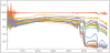
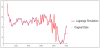
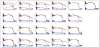
Our simulation is based on signal classication approach using discrete wavelet transform (DWT). A DWT-based linear (un) mixing system is designed specially for estimation. Using the wavelet transform, the original signal is represented by a set of wavelet transform coffiecients, and features are extracted from these coffiecients. Wavelet theory provides a good technique for signal approximation using scaled basis functions. The inverted data of the hyperspectral imaging illustrated in Figure 4. Note that the XY-axes ranges presented in Figures 4-11 are not refer to the actual wavelength and reflectance ranges of this study. The ranges presented here came from the ListLinePlot command using Mathematica software that plots a line through the points {1, y₁}, {2, y₂},..., {647, y₆₄₇} where the set {y₁, y₂,..., y₆₄₇} presenting the spectral image data of the binary system of Na₂SO₄-MgSO₄.

Figure 4: Hyperspectral imaging (un)mixing data.

Figure 5: Simulation using Lagrange interpolation.

Figure 6: A closer view of the simulation using Lagrange interpolation.

Figure 7: Simulations using Haar and Daubechies wavelets thresholds, respectively.

Figure 8: A closer view for the simulations using Haar and Daubechies wavelets thresholds, respectively.

Figure 9: Haar wavelet simulation of the whole spectra.

Figure 10: Splitting the the binary system of Na₂SO₄-MgSO₄ using the vector projection method.

Figure 11: Splitting the whole spectra using the vector projection method.

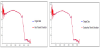
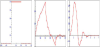
The first approach utilized the Lagrange Interpolation Technique. The simulation using Lagrange interpolation is illustrated in Figure 5. A closer view of the simulation using this approach is depicted in Figure 6.

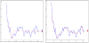
The second approach is by using wavelets interpolation, the first will be done using Haar wavelets and the second by Daubechies wavelets. The simulations using these functions are depicted in Figure 7 and 8.

4. Conclusion

The study used two approaches 1) semantic one by tracing the diagnostic spectral features such as the location, shape and depth of the band for certain endmembers and through study the association of the diagnostic feature between the mixed spectra and their endmembers (semantic or diagnostic approach), 2) mathematically through wavelet approach that simulate and unmix the reflectance spectra. To this end, a one-dimensional threshold method for hyperspectral images has been proposed based on Lagrange interpolation and discreet wavelet threshold denoising method. The performance of Lagrange interpolation method and the wavelet approach based on Haar and Daubechies threshold methods to simulate Na₂SO₄-MgSO₄ binary system yielded satisfactory results. Vector projection method was used successfully to split the hyperspectral data as a sum of two data functions that simulate it.

5. List of Symbols

P(x) A polynomial of degree n
ℝ The set of real numbers
ℤ The set of integers, 0,±1,±2,...
h₀[k] Sequence of real number where k∈ℤ
∑ k=1 n x k The summation of the values of x_k where k∈ℤ
∑ k∈ℤ x k Innite summation
Ψ The wavelet function
∫ f(x)dx The integral operator of the function f
∏ j=1 n x k Finite product
L 2 (ℝ) The space of functions f:ℝ↦ℝ for which ∫ f 2 < ∞
T_af(x) The translation operator by a of the function f
Df(x) The dilation operator of the function f dend by 2 f(2x)
Ψ l,j,k Ψ l,j,k (x)= D j T k Ψ l (x)= 2 j/2 Ψ( 2 j x−k)
a∙b The dot product of a and b
[a,b] The set of real numbers between a and b
X[0,1)(x) The characteristic function of the set [0, 1]
〈 f, Ψ l,g,k 〉 The inner product between f and Ψ l,g,k
X(Ψ) The wavelet system

Competing Interests

The authors declare that they have no competing interests.

Acknowledgments

We are very grateful to the anonymous referees valuable comments and suggestions.