


1. Introduction
In the last two decades, the use of atomistic/molecular simulations based on electronic structure calculations have become an extremely powerful tool to complement and reinforce results obtained in laboratory and in-field experiments. This did not only happen because of the development and implementation of new simulation methodologies, but also because the ever-growing computational power of work stations and high performance computers allowed dealing with more complex models and problems.
In particular, those research fields in Earth and Environmental Sciences where laboratory experiments are difficult, or even impossible to be performed, have deeply benefited of the use of this type of simulations. For instance, due to the extreme working conditions required in high pressure-temperature experiments resembling the environment of the Earth’s core, electronic structure simulations have been a great help to better understand elastic properties at the core of our planet [1-4]. Another example of atomistic simulations in environmental science is in the field of nuclear waste management, where direct experiments require very expensive and specialized equipment [5-7].
The most frequently used method in atomistic simulations based on electronic structure calculations is Density Functional Theory (DFT) [8]. This method, derived from quantum mechanics, is based on the Hohenberg-Kohn theorems which state that the total energy of the ground state is a unique functional of the electron density, and the functional that derives this energy gives the lowest energy if and only if the input density is the true one for the ground state. Therefore, in DFT calculations one has to compute the electron density of the modelled systems. This is an extremely expensive simulation, limited nowadays to models of up to 1000 atoms at most in large supercomputers, since the computational costs scale in a factor range of 3-4 respect to the number of atoms in the simulation (N3-4). As an example, the Archer supercomputer in the UK spent 60% of its computational capacity performing DFT simulations in the last month [9].
An alternative to massive parallelization of DFT codes in High Performance Computing (HPC) centers or supercomputers is using new processors that have this parallelization performance incorporated, and this is exactly what Graphic Processors Units (GPUs) do. GPUs allow the calculation of many operations in parallel environment with a shared memory structure and exchanging information with a CPU that controls the flux data in the DFT calculation.
Therefore, in this mini-review we present some recent advances performed in GPUs utilized in the field of DFT simulations, and the success in acceleration of the simulations performed in relatively small computer systems thanks to the CPU/GPU technology. This mini-review focuses on how CPU/GPU systems help accelerate DFT simulations from a didactic point of view, especially intended for those researchers and scientists not used to the difficulties derived from complex computational codes, where different architectures and memory sharing programming strategies have to be taken into account. Therefore, for those who need a greater detail on GPU programming, we recommend they search information for the specific GPU cards and their manufacturers.
2. Factors to Take into Consideration
2.1 Accuracy
Before commenting about the acceleration that GPU can provide to DFT codes, another consideration must be taking into account, i.e. the accuracy of the results. One of the first challenges found to move DFT calculations from standard CPU systems to combined CPU/ GPU when the first GPU cards appeared was that those cards were working on single-precision floating points. Although single precision calculations are enough in many scientific fields as in graphics generation or in artificial intelligence development, in order to obtain accuracies in the range of 1 kcal•mol-1 and avoiding convergence problems in numerical evaluations of the DFT energies, singleprecision calculations are not enough. Until the first double-precision GPU cards were developed (in 2009 NVIDIA put in the market the double-precision 64 bits GT200 GPU cards), the requirements for DFT calculations were not met.
Nevertheless, this was only the first step to overcome in terms of accuracy for the DFT calculations in CPU/GPU systems. During DFT calculations, several libraries are used to compute Fast Fourier Transformations (FFTs), matrix diagonalizations, and other operations. Those libraries have been used and tested for decades in the CPU versions of DFT codes, but it cannot be said the same for their counterparts in the GPU case. Fortunately, accuracy tests performed on different DFT-based codes as OCTOPUS [10] or VASP [11] have shown that the differences between the pure CPU and the CPU/GPU results are negligible in terms of accuracy respect to the chemical accuracy in DFT methods (<1 kJ•mol-1).
2.2 Memory transfer and sharing
One of the time consuming parts of DFT codes is the memory transfer and results sharing between nodes and CPUs. This step cannot be avoided since new data is required for posterior new calculations in the code. In High Performance Computer (HPC)clusters,the nodes are connected via infinibands to maximise the information speed exchange and, in particular, DFT codes use the Message Passing Interface (mpi) protocol. However, the communication between nodes is a relatively slow step, therefore, if one can perform simulations in less nodes or in a single node thanks to the CPU/GPU combination, the simulation can benefit from two factors: the GPU acceleration and the fact of supressing or reducing the mpi communication requirement.
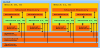
However, we are yet to discuss the memory configuration of CPU/ GPU architecture. The node or host has the main computation memory for the CPUs and the different threads if the multiprocessors can access it for calculations. Nevertheless, the GPU card also possesses its own layers of memory. Figure 1 shows the CUDA memory model of a GPU grid. CPU and GPU communicate the information required through the global and texture memory of the GPU, which is both accessible from the CPU and the GPU. However, this communication is still taking time, and in the programming process of the DFT codes one has to take this into account, avoiding the CPU/GPU information transmission unless necessary. During all the operations performed in the GPU, only the local memories of some racks of threads of the GPU, or if necessary exchanging information with other racks of threads in the same GPU card, via the shared memory. Final results, when required by the CPU to continue the overall calculation, are copied from the GPU shared memory to the Global memory and then accessed by the CPU.
All of these processes of accessing and copying can be asynchronically performed, although one has to balance properly the CPU/GPU calculations and their memory exchange to avoid this step becoming the bottleneck of the calculations [12].
2.3 CPU vs GPU workflow
During the DFT calculation, most of the computational time is spent in obtaining the electronic density which minimizes the energy for the given electronic potential, with both local and non-local contributions. Therefore any step performed in this evaluation that can be massively parallelised, will be largely benefited from the GPUs grid. These operations imply routines that convert the wave-functions from real space to reciprocal space (FFT transformations), matrices diagonalization, etc. One has also to take into account that this is true for very large blocks of data. GPUs can perform multiparallel calculations on large data blocks, but their acceleration is small if the data blocks are not large enough. Those processes with small data blocks and that require linear evaluations will be still better evaluated in the CPUs.
One example of this is the Wave Function evaluation in periodic DFT codes, which is performed in the HPC CPU systems in the reciprocal space and requires blocks of data that are relatively small, which are parallelised over the different wave functions (or orbitals) in the different CPUs. However, this changes when using GPUs; in order to take advantage of the large parallelism of these computational systems, calculations are performed in the real space and large data blocks are allocated in the GPUs. In doing so, the wave function evaluation becomes much slower than in the CPU case, but the rest of operations such as FFT transformations, diagonalizations or density matrix evaluation become much faster (see Figure 8.5 on reference 12).
With this example we want to point out that the GPU implementation of the codes is not straight-forward. The decision of which subroutines must be passed to the GPU must be done carefully and the different architectures of CPU and GPU parallelisation may need a clever approximation to modify these subroutines and how they share the work between the different threads of the GPU card [13,14].
2.4 CPU/GPU ratios
Another important factor in the acceleration process of the DFT codes using GPU cards is the ratio between the CPU processors and how many GPU cards they require. This simple question can be difficult to respond to it as depends on the codebeing used and the architecture of the CPU and GPUs used in the simulations. This ratio is also important in terms of node costs and the parallelization of the codes. One CPU can be composed of several processors, and at the same time they can have access to one or several GPU cards, whose work must be properly distributed. Although not a general rule, it has been found for VASP [15] and PETOT [13] codes that the largest accelerations in the DFT calculations are found ratios of CPU/GPU 1:2 to 1:4.
3. Conclusions
3.1 Acceleration results
As commented in previous sections, the acceleration factor obtained in the CPU/GPU system will depend on many factors: the architecture and the interconnections of the nodes of a cluster, the internal architecture and ratio in the CPU/GPU system, the parallelization scheme of the code used for calculations, and the type of DFT simulations that the code is performing in any case. In particular, we are going to comment results on VASP [11,16], PEtot [13] and OCTOPUS [10] codes. In VASP and PEtot codes, the Kohn- Sham equations are solved making use of a development of the oneelectron wave function in a basis of plane waves, and the effect of the core electrons on the valence electrons is normally described by ulstrasoft pseudopotentials or the projector augmented wave method.
The use of plane waves makes that the calculations are performed on the reciprocal wave vector space, with multiple FFT transformations. As previously commented, this step can be extremely accelerated with the combination of CPU and GPUs computation. On the other hand, OCTOPUS uses a real-space approach, where the fields in the Kohn- Sham equation are discretized in a grid (the effect core electrons on valence is treated as in the case previously mentioned). Because of the use of grids in real-space implies computing all the elements of the Kohn-Sham equations in parallel, this implies large blocks of data, and the corresponding parts of the codes can be computed in the GPU unit.
In VASP code calculations, accelerations values between 3 and 8 times have been obtained, depending on the subroutines used, different architectures and different chemical compounds used for the simulations [11,16]. Other similar codes have reported even larger accelerations, 10x for OCTOPUS [10] or even up to 20 times with respect to the CPU version for PEtot code [13],and even more in codes that combine DFT and Molecular Mechanics methodologies (QM/MM methodology), where the benefits are even larger, from 22 to 44 times faster than the pure CPU version [17]. Therefore, this clearly shows that spending time in moving the CPU versions of those codes into the GPUs is beneficial for time saving in the calculations.
3.2 Are the CPU/GPU systems worth the money?
Once the acceleration obtained with the CPU/GPU versions of the DFT codes with respect to the CPU versions is known, one can wonder whether this acceleration makes the extra money used to buy the GPU systems worth it. The addition of GPU cards to the CPU can mean that the price of the node doubles, or even more. Therefore one has to compare if the CPU/GPU systems is economically better than a cluster of CPUs connected by an infiniband. And the answer is yes.
First, the amount of money required in the infiniband will decrease or even disappear in reducing the number of nodes. Second the number of nodes will also decrease. Because one gets with the GPU systems accelerations much beyond 3 (up to 20-40 times), duplicating the price of the node is less than the acceleration obtained, and therefore, the price/performance ratio decreases.
This can be especially useful in relatively small computing clusters. With new CPU/GPUs configurations one can perform calculations that were previously restricted to very large HPC systems, but with less nodes and therefore, avoiding the transmission of information required among them, which slows down the calculations between nodes.
Competing Interests
The authors declare that they have no competing interests.