


1. Introduction
In Japan NO2 and NOx nearby heavy traffic road can still be locally high [1] in spite of continuously strengthened car emission regulation. For example, though the environmental standard for NO2 in Japan, which is defined as that the daily average value of one-hour- NO2 concentration should be lower than 60 ppb, is generally satisfied at observation sites operated by local and national governments, in Aichi Prefecture the maximum one-hour-NO2 was larger than 80 ppb (with its largest value of 107 ppb) at 6 sites of total 23 roadside sites for one year from April of 2014 to March of 2015, and the maximum onehour- NOx (=NO + NO2) similarly exceeded 200 ppb (with its largest value of 489 ppb) at 11 sites [1]. Therefore an appropriate method is required to reduce the local pollution without excess energy use and hence excess running-cost. To decrease high NO2 concentration at roadside with heavy trafic, mainly two methods were tested in Japan for the last 20 years; one is TiO2 coated panels set at road sides, and they were used, for example, on Route 43 in Osaka City, Japan. The panels trap NOx on their surface and oxidize NO and NO2 to NO3-(HNO3). The other one is to use specially prepared soil layer. The method was applied, for example, on Route 43 in Nishinomiya City, Hyogo Pref., Japan. Micro-bial actibity in the soil layer scavenges NOx in the polluted air which is pumped into the soil layer after oxidation of NO to NO2 by generated ozone. Though these two methods showed some effects on reduction of high NO2 concentration, their shortcomings such as relatively low performance on decreasing ambient NO2 concentration, high running cost, etc. were also appeared [2].
This paper evaluates a new method which uses fences filled inside with activated carbon fibers (ACF) to decrease high NO2 and NOx concentrations in urban atmosphere without excess energy use. Activated carbon fibers (ACF) is known as highly effective material to remove pollutants from flue gas [3-5], and from ambient atmosphere [6,7]. The idea of this paper is to utilize ACF as material filled inside in the fences placed at road side. In this situation pollutants-rich air in road space moves with natural-and car-induced- winds so as to contact with- and flow through-the ACF fences. And the ACF layer removes NOx from the polluted air. This “energy-free” equipment for air pollution reduction is proposed, and its performance is numerically evaluated in hypothetical road and wind situation.
2. Governing Equations
For evaluation of the performance of ACF fences in NOx concentration abatement, a set of non-thermal flow equations and advection-diffusion equation of air pollutant were applied with a standard k-ε turbulence model [8,9]. ACF fence was treated as porous media [10-12]. The following equations were numerically solved with a control volume method using software of CFX5 [13].
Continuity equation:
Momentum equation:
where Bi is the resistance to the flow in the porous media (ACF fence):
Advection-diffusion equation of air pollutant:
Equation for turbulent kinetic energy, k:
Equation for dissipation of turbulent kinetic energy, ε:
Shear production term of turbulent kinetic energy, P in Eqs. (5) and (6):
Eddy diffusivity:
Parameters (standard k-ε model):
The symbol γ and Kij in the equations denote the volume porosity and the area porosity tensor, respectively. Kij accounts for directivity of the flow in the porous media (i.e., ACF layer in the fence) and was assumed as a unit tensor. The volume porosity γ represents a ratio of the cavity volume in thecomputational grid cell volume.The true density of ACF is about 1.7~2.2 g cm-3. Since we use our standard packing density of ACF in the fence = 0.066 g cm-3, can be calculated as about 0.96 ( 1-0.066/1.7) with the true density of ACF= 1.7 g cm- 3;thus we assumed .Rc in Eq. 3 and kc in Eq. 4 are two important parameters characterizing ACF fence module, and will be discussed in chapter 3.
A similar system of equations but different resistance formulation and no chemical reaction was applied elsewhere [15].
3. Removal rate coefficient, kc and resistance coefficient, Rc
3.1 Removal rate coefficient kc
NOx (=NO + NO2) removal by ACF can be influenced by several factors such as type of ACF, packing density of ACF, and coexistence of other gases [6]. For simplicity, we assumed the first order removal reaction based on the laboratory experimental data [6,7]. The experiments were conducted by sucking ambient polluted air through glass tube packed with ACF. The reaction rate coefficient kc can be evaluated from Eq. (11) by using NOx (and NO2) concentrations measured at inlet and outlet of the glass tube with passing time through the ACF layer of sampled air:
From Eq. (9), the reaction rate constant can be obtained as:
where [NOx]i and [NOx]o denote NOx concentration at inlet and outlet of the glass tube packed with ACF, respectively, and t is the time required for the NOx containing air passing through the ACF layer. By using experimental data [6,7], the rate coefficient kc in Eq. 4 was determined for packing density of ACF at 0.066 g cm-3 (corresponding to γ=0.95) as:
kc for NOx: 1 ~ 2 s-1 and for NO2: 2 ~ 3 s-1
In numerical experiments, we varied as a parameter ranging 0 ~ 3 s-1.
3.2 Resistance coefficient Rc
Drag of ACF layer (assumed as a porous media) to the flow is included in Bi in Eq. (2). In this study, Bi was experimentally determined as Eq. (3). When air passes through a porous media, the media’s resistance is expressed as Eq. (12) [15].
where ρ is the air density, L is the length of porous media, ν is the kinematic viscosity of air, V is the flow velocity averaged over the cross section of porous material, p1 and p2 are the pressure of the air flow after and before the porous media, respectively. The parameters of α and in Eq. (12) are to be determined. Using laboratory experiments [7], we found that Eq. (12) can be rewritten so that only the first term is remained on the right hand side. Thus we obtained the following relation by comparing Eq. (3) with the simplified Eq. (12).
Coefficient Rc in Bi (Eq. 3) was estimated by utilizing the laboratory experimental data [7] of pressure drop and flow velocity in ACF layer on the far right hand side in Eq. (13). Obtained Rc values for two types of ACF fence-module, panel type and slit-type module (Figure 1), were as follows:
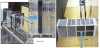
In the panel type module, ACF was packed in 10cm thick with the density of 0.066 g cm-3, while in the slit type module, many thin panels of 0.6 cm thick with the same ACF packing density were placed parallel each other with a distance of 1.6 cm between adjacent thin panels [7,11].
4. Calculation Domain and Simulation Conditions
4.1 Calculation domain
Two types of calculation domain were assumed: one is for double fences placed at both sides of the road as shown in Figure 2, and the other one is for single fence set only at lee side of the road. Pollutant was assumed to be discharged from the road surface as constant volume source with its height 1 m from the road surface; the source strength was 6.7x10⁻⁸kgm-3s-1; it should be noted that calculated concentrations can linearly change with this source strength. In the calculation, inside of each fence of 10 cm thick was resolved with a grid size of Δx= 2 cm for main stream direction (x axis).
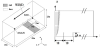
Figure 3 shows grid system for the double-fences. Thickness of each fence was 10 cm, and was resolved with 2 cm grid size for x direction. The grid size for x direction was smaller near the fences and was gradually enlarged up to 1 m. For z direction, the grid size was 20 cm from ground to the top of the fence, and then gradually increased up to 1 m long. For y direction, the grid size was set constant at 1 m.
Where we assumed that the roughness length zo = 0.23 m, and U1 at z=10 m is 1.8 ms-1 with Karman constant =0.4; then the friction velocity u* =0.19 ms-1 is estimated; Eq. (14) gives, for example, U1 =0.7, 1, 1.4 ms-1 at z=1, 2, 4 m, respectively.
Since the whole calculation domain is submerged in the surface layer, we set minimum values for k and so that the lower bound for diffusivity is assured in the road space: that is, the lowest diffusivity is 0.04 m2 s-1 for outside of the fences, and is molecular diffusivity for inside of the fences. Actually, the minimum calculated diffusivity was about 8.4x10⁻⁵ m2 s-1 at the inside of the ACF fences which is several times larger than the molecular diffusivity.
5. Results and Discussion
For both double- and single-fence cases, performance of the
ACF fences in NOx concentration reduction at the roadside was
numerically evaluated. Two parameters characterizing ACF fence, kc
and
Small
It should be noted that Eq. (4) for NOx transport and chemical removal is linear with respect to its concentration, C, and thus calculated concentration linearly responds to given emission source strength; this means the results of NOx concentration fields and profiles appeared in the following sub-sections can be interpreted following to various emission source scenarios; for example, if emission source strength from road is half of the current calculation (see sub-section 4.1), predicted concentrations will be half of the values shown in this study.
6. Calculated NOx field
6.1 Double fences
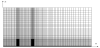
Figure 4 shows calculated NOx concentration field; the left column,
Figure 4 (a, c, e), is for the smaller resistance case (“slit” type fence
module) with
In the case of kc = 0(no chemical removal of NOx), the concentration
fieldsin downstream area where x > 20 m show almost same pattern
for
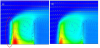
Differences between Figure 4(a,b) and Figure 4(c–f) show NOx removal effect by ACF fences. Though we discuss the NOx reduction quantitatively later in the subsection 5.3, large decrease in NOx concentration in the area downstream of the road (x> 20 m) can be seen in Figure 4(c-f); moreover, the decrease is more eminent in the lower height near the ground surface; for example, at the ground level of x=40 m, the NOx concentration at 170 ppb with no-ACF effect (Figure 4b) decreases to 110 ppb with kc=1 (Figure 4d) and 95 ppb with kc=3 (Figure 4f).
In the active ACF cases with 1 and 3 Figure 4(c-f), NOx concentration in downstream area (x>20 m) is always higher in the lower resistance coefficient of =400 (Figs. 4c, e) than the =3700 case (Figure 4d and Figure 4f). This difference indicates lowerNOx removal efficiency of the ACF fence with =400 in the road space; that is, as described above, contact of NOx-rich air with the ACF fence is suppressed by the clean air introduced from outside of the road (Figure 5a) because of lower resistance of the =400 ACF fence to the flow. Finally, it can be said that Figure 4 and Figure 5 show importance to utilize high concentration zone, formed by road structure such as fence, for effective removal of pollutants.
6.2 Single fence
Figure 6 shows calculated NOx fields of the single fence case. The
largest difference found in Figure 6(c-f) (single fence) and Figure
4(c-f) (double fences) is that in contrast to the double-fence case, in
the single fence case the smaller
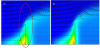
Another observation is that Figure 6 for the single fence cases shows lower NOx concentration in the downstream area than Figure 4 for the double-fence cases. This can be attributed to the flow characteristic that in the single fence cases, circulating flow is not formed in the road space and thus large upward flow is generated over the single fence placed on the downwind side of the road as shown in Figure 7; in this situation, polluted air mass in the road space tends to be higher lifted over the ACF fence, leading lower NOx concentration in the downstream area, in particular, at lower heights near the ground as shown in Figure 6.
6.3 Evaluation of NOx concentration reduction by ACF fence
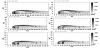
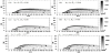
Figure 8 and 9 show vertical profiles of calculated NOx at 10 m downwind from the leeward side fence (namely, at x=30 m and y= 12 m in Figure 2) for the double- and single-fence case, respectively.
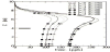
Figure 8 (“double-fence” case) demonstrates that ACF fences can
reduce near-surface NOx concentration at the roadside by 15 ~ 40%
than the no-removal activity fence (kc=0; open and solid circles in
Figure 8). Since difference in NOx concentration between cases with
kc=1 (symbol “triangle”) and 3 (symbol “square”) is relatively small,
NOx removal process by ACF is thought to be rather diffusionlimited
if kc value exceeds around 1 s-1. Moreover, it is suggested that
fence of larger resistance, which corresponds to “panel” type module
with
Also in single-fence situation, it is shown that the ACF fences can
cut NOx concentration by 30 ~ 55% (Figure 9). In contrast to the
double-fence case, that fence with small resistance (
Moreover, it is shown that the single-fence case (Figure 9) gives rather smaller NOx concentration at lower heights, for example, below 4 m than the double-fence case (Figure 8). This is again attributable to the enhanced upward motion over the leeward fence in single fence cases (Figure 7) compared with double-fence cases (Figure 5), leading to higher vertical transport of the pollutant and hence lower concentration near the ground surface in the leeward space of the road.
7. Summary and Conclusions
In this study, a new method to reduce ambient NOx concentration without excess energy use was proposed and its performance was numerically evaluated. The method is to set a “porous” flow-through fence filled inside with ACF (Activated Carbon Fibers) along heavy traffic road. ACF is pre-treated carbon fiber [16] and highly effective in removal of NOx, SO2, etc. By using a control volume method, partial differential equations of flow, turbulence, and NOx transport were simultaneously solved to predict NOx concentration reduced by the double- and single-ACF-fence.
Two important parameters on the ACF fence were identified: one is
the resistance of ACF layer to the air flow, the resistance coefficient
-
in the double-fence case, high concentration zone is formed near
the ACF fence on upstream side due to the circulation generated in
the road space. In this case, the fence with higher ventilation (low
-
in the single fence case, on the other hand, smaller resistance of the
ACF fence is better for the pollutants’ removal, since higher pollutants’
flux through the ACF layer is expected with the ACF fence of low
- in both double- and single- fence cases, the process decreasing NOx concentration is suggested rather diffusion-limited if kc is larger than about 1 s-1, indicating frequency of the contact of polluted air with the fences is important.
8. Nomenclature
Bi = resistance to air flow in i direction by ACF layer defined in Eq.
(3), (L T-2)
C = dimensionless concentration of NOx in air in Eq. (4)
C1, C2, Cμ = parameters in the standard k-εmodel; the values are listed
in Eq. (9)
Kij, Kjk = area-porosity tensor of ACF layer in Eq. (1), (2), (4), (5), and
(6); unit tensor is assumed; for example, Kij= 1 for i=j, and 0 for i≠j.
k = turbulent kinetic energy in Eq. (5), (6), and (8), (L2 T-2)
kc = removal rate coefficient of NOx by ACF layer in Eq. (4), (10), and
(11), T-1
L = thickness of ACF layer in Eq. (12) and (13), L
[NOx ] = dimensionless concentration of NOx in air in Eq. (10)
[NOx]i= dimensionless concentration of NOx in air at inlet in Eq. (11)
[NOx]o= dimensionless concentration of NOx in air at outlet in Eq.
(11)
P = shear production term of turbulent kinetic energy in Eq. (5), (6),
and (7), (L2 T-3)
p = pressure of air in Eq. (2), (N L-2)
p1, p2 = pressure of air in Eq. (12) and (13), (N L-2)
Rc = resistance coefficient in Eq. (3), T-1
t = time, T
Ui= air flow velocity for i direction in Eq. (1), (2), (4), (5), (6), and (7);
i = 1, 2, 3 for x, y, z direction, respectively, (L T-1)
u* = friction velocity in Eq. (14), (L T-1)
V = air flow velocity in Eq. (12) and (13), (L T-1)
xi = coordinate axis; i=1, 2, 3 for x, y, z direction, respectively; for
example, x3 (= z) for vertical direction and positive for upward, L
z = vertical coordinate axis (= x3) in Eq. (14); height above ground
surface, L
z0 = roughness length in Eq. (14), L
9. Greek Letters
α = coefficient in Eq. (12) and (13). β = coefficient in Eq. (12).
Γt = turbulent diffusivity of pollutant in air in Eq. (4) assumed equal
to νt as in Eq. (8), (L2 T-1)
γ = volume porosity of ACF layer as assumed porous media in Eq. (3),
(4), (5), (6), and (13).
ε = dissipation rate of turbulent kinetic energy in Eq. (5), (6), and (8),
(L2 T-3)
κ = Karman constant in Eq. (14)
ν =molecular kinematic viscosity of air in Eq. (12) and (13), (L2 T-1)
νt = turbulent kinematic viscosity of air evaluated by Eq. (8), (L2 T-1)
ρ = air density in Eq. (2), (4), (12), and (13), (M L-3) σk, σε = parameters
in the standard k-ε model; the values are listed in Eq. (9)
Competing Interests
The authors declare that they have no competing interests.