


1. Introduction
In this article, the authors propose the use of the Least Square Method (LSM) as a procedure that can help us obtain a mathematical formula that can be used to complement, and if possible, better any of the models used so far, particularly, on the area of medicine. The LSM will be used to fit the curve of a graph from which we can generate a mathematical formula.
The procedure is a simple three-step process: first, collect the field data. Second, make a graph from the data obtained, and, as the third and last step, use the LSM to generate a mathematical formula. From the plot of this graph, after applying the LSM, we can generate a formula that can be easily taught and used worldwide without the need of having specialized workshops to teach the use and application of the formula.
2. Using the Least Square Method to Find the Equation of Covid-19 Curve Sample
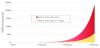
To illustrate the proposed methodology in a step-by-step fashion, we will use a real-life example to find the equation of the curve of COVID-19 behavior. The data was obtained from a New York Time Article, The Exponential Power of Now by Siobhan Roberts [1] with the graphic of Britta Jewell [2], of the Institute for Diseasing Model. Published on March 13, 2020. The objective is to obtain a graph to which we can apply the LSM to derive a mathematical formula that we can use, as indicated later, for several other purposes including the study of any variable of this or any other disease. As a caveat to the reader, the figures used in this paper are not at a true scale although the values shown are actual measurements; all figures are only used to convey shapes and procedures. Figure 1 illustrates a typical COVID-19 curve profile and its values.
2.1 Identifying the coordinates
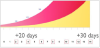
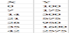
The coordinates of the graph were found by measuring the height of the curve at seven different horizontal intervals, as shown in Figure 2.
2.2 Choosing the curve’s form
After determining the coordinates, it was necessary to choose a curve that approximates the shape of the COVID-19 sample curve. Figure 3 shows the graphs of some of the most commonly used functions for fitting curves using the LSM [3].
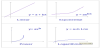
For this case, we chose the graph of the exponential function y = aebx (F1) because its mirror-image, about the horizontal axis of the graph. We will use the LSM to fit the exponential graph to the profile of the curve.
2.3 System of equations
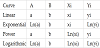
To obtain the coefficients a and b of the exponential function, LSM requires solving the system of equations F1 shown below. Table 1 explains the meaning of the different terms depending on the type of curve selected [4].
2.4 Rewriting the system
Substituting the exponential values into F1 we obtain
Where “n” is the number of coordinates previously obtained and whose values are shown in Table 2.
3. Solving the System of Equations
3.1 Calculating the individual terms [4]
In this example, n = 7 (the number of coordinates)
The summation of all Xs values is:
The summation of all the squares of the Xs coordinates is:
The summation of the logarithms of the Ys coordinates of Table 2 is:
The summation of all Xs coordinates multiplied by its corresponding Y logarithm is:
3.2 Substituting all terms in the System of equation F2
Performing the corresponding arithmetic operations, we obtain the following results:
3.3 Calculating the b coefficient
Solving the top equation of (F3) for Ln(a) give us
Replacing this value in the second equation of F3 we obtain:
Solving for the coefficient b from the latter equation results in
3.4 Calculating the a coefficient
To find the coefficient a, we replace the value of b in the second equation of the system F3 and solve for Ln(a). That is,
Raising e to value just obtained results in:
4. Equation of Covid-19's Curve
Following the procedure outlined we can rewrite the equation 1 using the coefficients a and b just calculated
Using the exponential equation previously selected (F1)
and substituting the coefficients, a and b we get the following function [5]
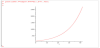
When we plot the latter equation into the Maple software the values of x initially obtained in Table 2, the graphic (Figure 4) obtained is very close to shape of the Figure 1. So, equation 1 approximates indeed the profile of the graphic.
5. Excel Workbook Test
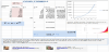
To improve the work we made a Microsoft Exce™ calculation spreadsheet with the LMS parameters (Figure 5). In the first column we placed the Xs coordinates. In the second one we can find Ys coordinates. The third column is the summation of all the Xs. The fourth column has the summation of all the squares Xs. The fifth, the summation of the logarithms of the Ys. And the sixth one, the product of each Xs by the logarithms of all the Ys.
Competing Interests
The authors declare that they have no competing interests.
References
- Roberts S (2020) The Exponential power of now. The New York Times. [View]
- Institute For Disease Modeling.
- Mujica J (1982) Infinitesimal Calculus with Analytic Geometry and Computing Applied to Audio.
- Hewlett-Packard, Standard Applications Pac HP-4C, 00041-90018 Rev D.
- McCracken DD, Dorn WS (1964) Numerical Methods and Fortran Programming.
- Maple Software plot.
- Kolb WM (1982) Curve Fitting for programmable calculators.