


1. Introduction
The popularity of the wireless local-area network (WLAN) has remarkably increased in both residential and working areas as inexpensive, flexible Internet access services [1,2]. Nowadays, WLAN services are available in plenty of public places including airports, shopping malls, stations, or streets. The wireless communication between an access point (AP) and a host makes WLAN flexible, scalable, and accessible compared with the wired LAN.
In WLAN, the distribution of users is mostly non-uniform and non-stationary [3]. The number of users or traffics appears to be unpredictable [4] since they are inclined to fluctuate depending on the time and day of the week [2]. Besides, the conditions of network devices and communication links may suffer from various factors, such as power shortages, device failures, bandwidth controlled by the authorities or weather changes [5]. For instance, a great number of developing countries such as Bangladesh and Myanmar often suffer from the unreliable and poor Internet access and discontinuities of electricity supplies [6,7].
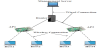
To solve the aforementioned problems, the elastic WLAN system using heterogeneous AP devices [8-10] was examined. To minimize the power consumption, the elastic WLAN system correspondingly controls the number of active APs according to traffic demands and device conditions. For the optimal control, we have proposed the active AP configuration algorithm which selects the minimum number of active APs that can satisfy the constraints in the system. Next, it will allocate the AP association to each host to balance the loads among active APs, and assign the channel to each active AP from the limited number of the non-interfered channels in order to minimize the overall interference. Three types of APs, namely dedicated APs (DAPs), virtual APs (VAPs), and mobile APs (MAPs), have been considered as shown in Figure 1.

In this paper, we propose the transmission power minimization extension in the active AP configuration algorithm to further reduce the energy consumption. The transmission power minimization is expected to lengthen the lifetime of the AP device [11]. In this extension, first, the previous active AP configuration finds the active APs, AP-host associations, and AP channel assignments, assuming the use of the maximum transmission power. Then, it minimizes the transmission power of each active AP such that it satisfies the minimum throughput constraint. The previous throughput estimation model [12] has been used to evaluate the throughput for each transmission power, where the model parameter values are obtained from extensive measurements.
The effectiveness of the proposed extension is verified through both simulations and experiments. In simulations, the WIMNET simulator [13] is adopted to estimate the throughput before and after applying the proposal. A small network topology and a large one are examined here, which model the real field in a building at Okayama University. In experiments, the elastic WLAN system testbed [10] is extended to conduct the proposed extension, where the real throughput is measured before and after the proposal. Both experiments confirm that the significant reduction of the transmission power has been achieved while the throughput performance was maintained.
The rest of this paper is organized as follows: Section II introduces related literature. Section III reviews our previous works. Section IV presents the transmission power minimization extension. Sections V and VI evaluate the proposal through simulations and testbed experiments, respectively. Finally, Section VII concludes this paper with future works.
2. Related Literature
In this section, we briefly introduce related literature in this paper.
[3] adopts a game theoretic approach to balance the loads among the APs. That is, the users associated with highly congested APs will be moved to less loaded APs for better throughputs. Although this approach can balance the load among APs, the user movement from one AP to another AP makes it impractical for real applications, because a host has to discover another suitable AP and move to the place, if it doesn’t succeed in receiving the required data rate or service from the associated AP.
[14,15] propose a load balancing approach among APs to mitigate congestions and fair distributions of users. Each host monitors the wireless channel qualities that it experiences from nearby APs and reports them to the network control center that determines the host and AP associations. Since the objective function of the proportional fairness is non-linear, its implementation is much more challenging, where detecting the bottleneck users and finding their normalized bandwidth are NP-hard.
[16] provides an algorithm to place several extension points for cellular networks such that the throughput capacity of WLAN is maximized. These extension points act as relay points between the APs and the hosts located at longer distances. Each extension point can receive the packets from the APs and deliver them to the hosts. In a conventional WLAN, the extension point is not used, because the multihop communications degrade the performance due to strong interferences among multi-hop links.
[17] presents an AP association approach to improve the network throughput while balancing the loads among APs. The authors investigate and evaluate a measurement driven framework with three objective functions in a dense WLAN; (i) the frequency/channel selection across the APs to minimize the noise or interference between neighboring APs, (ii) the user association by considering the load of the AP and the receiving signal strength, and (iii) the power control for each AP. While each of the three objective functions achieves its optimization objective individually, in certain cases, to apply all of them (channel selection, user association, and power control) will lead to the suboptimal performance. Moreover, the authors found that if all of them are randomly applied, it will degrade the performance. A host is initially associated with the AP that providessignal strength indicator (RSSI). Then, any host from an overloaded AP is migrated to a lightly loaded AP for balancing the load in the network.
[18] introduces a heuristic algorithm for the AP placement based on the user distribution on an indoor WLAN system. The authors have proposed a fuzzy C-clustering-based AP deployment strategy to maximize the user coverage and balance the load among the APs.
[19] examines an AP selection algorithm to maximize the throughput for a newly joining host in the multi-rate WLAN by moving the host towards the location of the desired AP.
[20-22] focus on the highest received signal strength indicator (RSSI) to select the AP association. However, the AP with the highest RSSI can be overloaded by a number of users, and thus, may not ensure the proper load balancing among APs.
[23] presents a smart AP solution to balance the loads across multiple Wi-Fi interfaces. Still, the implementation of this approach is difficult, since each AP must be equipped with multiple interfaces operating on different channels simultaneously.
A substantial amount of research works has been found in literature that focus on the power consumption at each active AP. Instead of simply powering on all access points with highest transmission-power, controlling the transmission power of APs on a large scale can minimize power consumption, distortion and increase the lifetime of APs [24,25]. For instance, [24] explores a genetic algorithm to control the power of each active APs in industrial wireless local area network (IWLAN).
3. Previous Works
In the section, we review our previous works related to this paper.
3.1 Elastic WLAN System
The elastic WLAN system has been studied to reserve the energy consumption by deactivating unnecessary APs while ensuring the required throughput performance for any host in WLAN. Figure 2 illustrates the topology of the system.
In the testbed of the elastic WLAN system, Raspberry Pi [26] is used for the AP and Linux PC is for the server and the host. The management server is adopted to manage and control the APs and the hosts by implementing the active AP configuration algorithm. This server not only has the administrative access to all the devices on the network, but also controls the whole system through the following three steps:
- The server explores all the devices in the network and collects the requisite information for the active AP configuration algorithm.
- The server executes the active AP configuration algorithm using the inputs derived in the previous step. The output of the algorithm contains the list of the active APs, the host associations, and the assigned channels.
- The server applies this output to the network by activating or deactivating the specified APs, changing the specified host associations, and assigning the channels.
3.2 Active AP Configuration Algorithm
The active AP configuration algorithm optimizes the configuration of the APs in WLAN including the selection of the active APs, their host associations and channel assignments. First, we introduce three different types of APs that we use in our AP configuration algorithm. Then we describe the problem formulation of active AP configuration algorithm.
- Heterogeneous AP Devices
The elastic WLAN system may use heterogeneous AP devices, namely dedicated APs (DAPs), virtual APs (VAPs), and mobile APs (MAPs), for the flexible implementation.
A DAP is a dedicated wireless AP that adopts the IEEE 802.11n wireless protocol and connects PCs to the Internet. A DAP assumes to be a commercial DAP. It has the coverage radius with around 110m and the transmission speed with around 120Mbps.
A VAP is a software-based AP using a personal computer (PC) with either Windows or Linux for the operating system as the platform. Many PCs can support the IEEE 802.11n protocol that has the transmission speed with around 54Mbps. Both DAP and VAP use wired Ethernet to access the Internet.
A MAP is a device that connects to the Internet through the 3G/4G wireless technology, such as a smart phone. For a MAP, the power supply is unnecessary because of the built-in battery. The transmission speed is around 30Mbps.
- Input and output
- Number of hosts: H
- Number of APs: N = ND + NV + NM. where ND, NV, and NM respectively represent the number of DAPs, VAPs, and MAPs
- AP ID: i = 1 to N
- Host ID: i = 1 to H
- Link speed of the ith AP to the jth host, sij (i = 1 to N, j = 1 to H): it can be estimated by the throughput estimation model described later in this Section.
- Number of non-interfered channels
- The set of active APs (DAPs, VAPs, and MAPs)
- The set of hosts associated with each active AP
- The assigned channel to each active AP
Inputs
Outputs
- Objective Functions
Three objective functions are defined for this algorithm. The first objective function E1 is defined to minimize the number of active APs (DAPs, VAPs and MAPs) in the network:
The second cost function in our algorithm is E2. It represents the minimum overall throughput of an AP, which is a bottleneck AP in the network. Then, we want to maximize the value of E2 to improve the overall throughput of the network. The cost function E2 is defined as follows:
where THj represents the average host throughput for the jth AP and is defined by:
where sjk represents the link speed between the jth AP and the kth host. Holding the first objective, our second objective function is to maximize the value of E2, the minimum overall throughput of an AP.
The third objective function E3 is defined to minimize the interference:
where ITi represents the interfered communication time for APi, Ti does the communication time for APi, Ii does the set of interfering APs for APi, and ci does the assigned channel to APi.
- Constraint
The minimum host throughput constraint is defined in this algorithm so that the throughput of every host exceeds the given threshold G on average when all the hosts are communicating simultaneously:
- Procedure of Active AP configuration algorithm
- First Phase
- Preprocessing: The link speed for each potential pair of an AP and a host is estimated by the throughput estimation model described later in this Section.
- Initial Solution Generation: An initial solution E1 is derived using a greedy algorithm [27].
- Host Association Improvement: The cost function E2 is calculated for the greedy solution using Equation (2). Then, this solution will be improved.
- AP Selection Optimization: The cost functions E1 and E2 are further jointly optimized in this phase by the local search under the constraints mentioned before [8] and [28].
- Link speed normalization: The fairness criterion will be adopted when the total expected bandwidth exceeds Ba. Ba represents the total available bandwidth of the network, which is determined by the external Ethernet bandwidth.
-
Termination check: When either of the following conditions is
satisfied, move to the second phase in 2:
- The minimum host throughput constraint is satisfied.
- All the APs in the network have been activated.
- Additional VAP activation: If VAPs are not selected for candidate APs, they will be selected as candidate APs, then return to Step Host Association Improvement.
The first phase of the algorithm selects the active APs and the host associations to minimize E1 and E2.
The first phase of our AP configuration algorithm selects APs and their host associations that minimizes the number of active APs and maximizes the minimum host throughput of the network. Using a greedy algorithm, the Initial Solution Generation stage provides the initial number of active APs, E1, and the hosts associated to these active APs. This solution can be poor, because the host associations are performed based on the AP coverages. Besides, this greedy algorithm cannot optimize the minimum host throughput, E2, which is our second objective.
In the Host Association Improvement stage, we improve the host associations among active APs that are found in the previous phase, by randomly changing the associations of the bottleneck hosts. This modification of host associations is carried out with a view to improve the overall throughput by optimizing the minimum host throughput. Although this stage can improve E2, it cannot guarantee to satisfy the minimum host throughput constraint by the current activate APs.
To satisfy this constraint, we apply the AP Selection Optimization stage. This stage optimizes the selection of active APs with AP-host associations to further minimize both E1 and E2 while satisfying the average throughput threshold G, using another local search method. If the average throughput constraint is not satisfied by the current number of active APs, this stage increases the number of active APs.
- Second phase
- Preprocessing: The interference and delay conditions of the network are represented by a graph.
- Interfered AP set generation: The set of APs that are interfering with each other is found for each AP.
- Initial solution construction: An initial solution is derived using a greedy algorithm.
- Solution improvement by simulated annealing: The initial solution is improved by the simulated annealing (SA) procedure with the constant SA temperature TSA for the SA repeating times RSA, where TSA and RSA are given algorithm parameters [9].
The second phase assigns a channel to each active AP to minimize E3.
- Third phase
- Initialization: The AP flag is initialized by 0(= OFF) for every AP. This flag is used to avoid repeating the same AP.
- AP selection: One OFF flag AP is selected to move its associated host to a different AP that is assigned a different channel.
- Host selection: One host associated with the selected AP is selected for the AP movement.
- Change application: Finally, the new associated AP is chosen for this selected host. We select the AP with the largest link speed among the APs. Then we calculate the cost function E using Equation 4, if the host is associated with this AP. If the new cost function E is equal to or smaller than the previous E, accept the new association then return to Step Host selection [9].
The third phase averages the load among the channels to minimize E3.
3.3 Throughput estimation model
The link speed or throughput between any AP and host depends on a variety of factors such as the modulation and coding scheme, transmission power, transmission distance. Therefore, the theoretical computation of the accurate link speed is challenging [8,29]. In our throughput estimation model, the receiving signal strength (RSS) at the host is first estimated using the log distance path loss model and then, the throughput is evaluated from the RSS using the sigmoid function [12].
- Received signal strength estimation
- Throughput estimation
First, the Euclidean distance d (m) is calculated for each link (AP/host pair) by:
where APx, APy and Hx, Hy does the x and y coordinates for the AP and the host respectively. Then, the RSS at a host from an AP is estimated using the log-distance path loss model:
where Pd represents RSS (dBm) at the host, P1 does RSS at the 1m distance from the AP when no obstacle exists, α does the path loss exponent, nk does the number of typek obstacles along the path from the AP to the host, and Wk does the signal attenuation factor (dBm) for typek obstacle.
From received signal strength Pd, the throughput is estimated by using the sigmoid function [12] as follows:
where sh represents the estimated throughput (Mbps) and, a, b, and c are constant coefficients.
4. Proposal of AP Transmission Power Minimization
In this section, we propose the AP transmission power minimization as the fourth phase of the active AP configuration algorithm.
4.1 Overview
To reduce the power consumption of the active APs, the transmission power minimization phase is added in the active AP configuration algorithm. That is, using the measurement results with different transmission powers, the parameter value in the throughput estimation model corresponding to the transmission power is found by applying the parameter optimization tool [12].
Then, the average host throughput for each transmission power is estimated using this model, and the least transmission power is selected to satisfy the minimum host throughput constraint for any AP. In the elastic WLAN system testbed, the transmission power of any Raspberry Pi AP is controlled by a Linux command.
4.2 Throughput measurements under transmission power reductions
The value of P1 in the throughput estimation model is found for each transmission power based on measurements, where P1 is related to the transmission power. The other parameters can be fixed at the ones with the full transmission power described later in this Section.
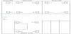
To observe the effect of the reduced transmission power in the throughput and estimate the value of P1 in the model, we conducted throughput measurements by using different transmission powers, namely, 5dBm, 10dBm, 20dBm, and 30dBm, for Raspberry Pi AP on the 3rd floor of Engineering Building-2 of Okayama University. The locations of the AP and the host in measurements are illustrated in Figure 3. Table 1 shows the adopted hardware and software in measurements.
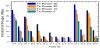
iperf 2.05 is used to generate TCP packets during the measurement [30]. Figure 4 offers the average throughput results among 10 measurements for each host location with the four different transmission powers. This figure indicates that (1) the host throughput becomes smaller when the transmission power is reduced, and (2) the throughput is not always proportional to the transmission power, because the modulation and coding scheme (MCS) [31] is changed stepwise.
4.3 P1 for different transmission powers
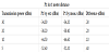
Then, the value of P1 in the throughput estimation model is estimated by applying the measurement results in Figure 4 to the parameter optimization tool [12]. As well, the other parameter values are fixed as in Table 2 at any transmission power.
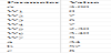
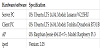
Table 3 shows the value of P1 for each transmission power. It is compared with the measured value of P1. This table reveals that both values are nearly the same, which confirms the accuracy of the throughput estimation model. However, for practical use of the proposal, it is necessary to reduce the number of throughput measurements required to tune the model parameters, which will be explored in future works.
4.5 Transmission power minimization
Using the throughput estimation model, the following procedure is proposed to minimize the transmission power of each active AP (let AP i here) that satisfies the minimum host throughput constraint, as the fourth phase of the active AP configuration algorithm. To improve the accuracy while reducing the computation time, the throughput is first estimated at an equal interval of the transmission power using the throughput estimation model. Then, the throughput at an arbitrary transmission power is obtained by the interpolation of the results at the two adjacent powers. We calculate the average host throughput that should be greater or equal to the throughput constraint G as follows:
-
Calculate the link throughput between AP i and its associated
host j, namely
-
Calculate the corresponding average host throughput for AP i,
-
Calculate the average host throughput for AP i,
-
if
-
else if
-
else if
-
else
-
if
-
Determine the minimum transmission power TXi that satisfies
the average host throughput constraint by:
-
if
-
else if
-
if
5. Evaluations by Simulations
In this section, we evaluate the proposed transmission power minimization through simulations in two network topologiesusing the WIMNET simulator [13].
5.1 Simulation platform
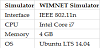
Table 4 shows the adopted hardware and software in simulations while table 5 provides the parameters in the WIMNET simulator.

5.2 Simulation in small network topology
First, the small network topology in Figure 5 is considered in simulations. It basically models the third floor of Engineering Building-2 in Okayama University. 15 hosts and six APs are regularly distributed in the corridor and rooms with 7m × 6m and 3.5m × 6m. G = 10Mbps and Ba = ∞ are adopted for the minimum host throughput constraint and the bandwidth limit constraint, respectively.
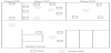
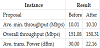
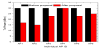
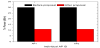
Table 6 shows the simulation results where the average minimum host throughput, the overall throughput, and the average transmission power is summarized. The results indicate that the proposal can reduce the transmission power by 26.13% while satisfying the minimum host throughput constraint and keeping the overall throughput before applying the proposal. Figure 6 compares the transmission power in each AP before and after the proposal. This figure implies that it can reduce the transmission power significantly while maintaining the performance, which confirms the effectiveness of the proposal.
5.3 Simulation in large network topology
Next, the large network topology in Figure 7 is considered, which has the same size as the small network topology. 40 hosts and 18 APs are allocated. For the minimum host throughput constraint, G = 10Mbps is adopted.
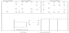
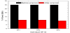
Table 7 reveals the simulation results, which indicate that the proposal reduces the transmitting power by 51.20% in the large topology. Figure 8 shows the transmission power reduction in each AP by the proposal. Once more, it was observed that the proposal has reduced the transmission power prominently while keeping the throughput performance.
6. Evaluation by Experiments
In this section, we evaluate our proposal through experiments using the elastic WLAN system testbed [10] in two buildings at Okayama University.
6.1 Experiments in Engineering Building-2
First, the third floor in Engineering Building-2 is adopted in experiments. Two scenarios are considered using a different number of rooms. Each room has 7m×6m size, where one Raspberry Pi for the AP and two Linux PCs for hosts are allocated. Then, two rooms are used in 2×4 scenario in Figure 9, and three rooms are in 3×6 scenario in Figure 10.
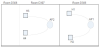
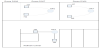
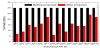
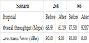
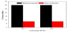
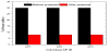
Table 8 compares the overall throughput and the average transmission power before and after applying the proposal in two scenarios. The overall throughput is similar between them, whereas the transmission power is reduced greatly by the proposal. Figure 11 and Figure 12 show the transmission power change at each AP.
6.2 Experiments in graduate school building
Next, the second floor in Graduate School Building is adopted in experiments with two scenarios. In 2×4 scenario, one room with 9m × 5.5m size is used, where two Raspberry Pi APs and four hosts are allocated, as indicated in Figure 13. In 3×6 scenario, additionally, one AP and two hosts are allocated in another room with 3.5m × 5.5m size, as shown in Figure 14.
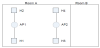
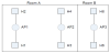
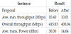
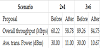
Table 9 compares the overall throughput and the average transmission power before and after applying the proposal. Figure 15 and 16 show the transmission power at each AP namely, the overall throughput is similar between them, whereas the transmission power is reduced significantly.
7. Conclusion aand Fiture works
In this paper, we proposed the transmission power minimization extension in the active AP configuration algorithm to further minimize the power consumption in the elastic WLAN system. The parameter values of the throughput estimation model for different transmission powers at an AP were derived based on measurement results. The effectiveness of the proposal was validated through simulations with the WIMNET simulator and experiments using the testbed in several network scenarios. In future works, we will reduce the number of throughput measurements required to tune the model parameters, and evaluate the proposal using the elastic WLAN testbed in various network fields and topologies.
Competing Interests
The authors declare that they have no competing interests.