


1. Introduction
The analysis of shapes and shape variation is of great importance in a wide variety of disciplines. Initially in 1917 D’Arcy Thompson [1] studied the field of geometrical shape analysis from a biological point of view. Intuitively it is especially interesting for biologists since shape is one of the most concise features of an object class and may change over time due to growth or evolution. The problems of shape spaces and distances have been intensively studied by Kendall [2] and Bookstein [3] in a statistical theory of shape. We follow Kendall [2] who defined shape as all the geometrical information that remains when location, scale, and rotational effects are filtered out from the object. Sometimes it is also interesting to retain the size of the objects, but we will not consider this case here. In most applications this invariance is not given a-priori, thus it is indispensable to transform the acquired shapes into a common reference frame. Different terms are equivalently used for this operation, i.e. superimposition, registration, and alignment. Only if the shapes are aligned, it will be possible to compare them in order to describe deformations or to define a measure distance between them.
Bookstein geometrically analyzed shapes and measured their change in many biological applications, e.g. bee wings, skulls, and i.e. human schizophrenia brains [4]. To give an example, with his morphometric studies he found out that the region connecting the two hemispheres is narrower in schizophrenic brains as in normal brains. In digital image processing the statistical analysis of shape is a fundamental task in object recognition and classification. It concern applications in a wide variety of fields, e.g. [5].
2. The Problem of Alignment of 2-D Shapes
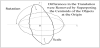
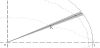
Consider two shape instances P and O defined by the point-sets pi ε R2, i= 1,2,...,Np and ok ε R2, k=1,2,...,N0 respectively. The basic task of aligning two shapes consists of transforming one of them (say P) so that it fits in some optimal way the other one (say O) (see Figure 1).
Generally the shape instance P={pi} is said to be aligned to the shape instance O={ok} if a distance d(P,O) between the two shapes can not be decreased by applying a transformation ψ to P. Various alignment approaches are known [6-12]. They mainly differ in the kind of mapping (i.e. similarity [8], rigid [13], affine [14]) and the chosen distance measure. A survey of different distance measures used in the field of shape matching can be found in [15].
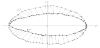
For calculating a distance between two shape instances the knowledge of corresponding points is required. If the shapes are defined by sets of landmarks [16,17] the knowledge of point correspondences is implicit. However at the beginning of many applications this condition is not hold and often it is hard or even impossible to assign landmarks to the acquired shapes. Then it is necessary to automatically determine point correspondences between the points of two aligned shapes P and O, see Figure 2.
One of the most essential demands on these approaches is symmetry. Symmetry means obtaining the same correspondences when mapping instance P to instance O and vise versa instance O to instance P. This requirement is often bound up with the condition to establish one-to-one correspondences. This means a point ok in shape instance O has exactly one corresponding point pk in shape instance P. If we compare point sets with unequal point numbers under the condition of one-to-one mapping then it is clear that some points will not have a correspondence in the other point set. These points are called outlier.
Special problems arise if we have to align shapes that are very different, for example aligning concave to convex shapes. In these cases it is indispensable to take into account the order of the point-sets and to enforce legal sets of correspondences, otherwise the calculated distances are incorrect. This paper presents our novel algorithm for aligning arbitrary 2D-shapes, represented as ordered point-sets. In our work natural shapes are acquired manually from real images. The object shapes can appear with varying orientation, position, and scale in the image. The shapes are arbitrary and there is nothing special about them. They might have a great natural variation. They also might be very similar or very dissimilar. They even might have concave or convex shapes. The algorithm establishes symmetric and legal one-to-one point correspondences between arbitrary shapes, represented as ordered sets of 2D-points and returns a distance measure which runs between 0 and 1.
3. Related Work
The problems of shape spaces and distances have been intensively studied [3,2] in a statistical theory of shape. The well-known Procrustes distance [8,16] between two point-sets P and O is defined as the sum of squared distances between corresponding points
where R(θ) is the rotation matrix, μP and μO are the centroids of the object P and O respectively, σP and σO are the standard deviations of the distance of a point to the centroid of the shapes and NPO is the number of point correspondences between the point-sets P and O. This example shows that the knowledge of correspondences is an important prerequisite for calculation of shape distances.
There has been done a lot of work which concerns the problem of automatic finding point correspondences between two unknown shapes. Hill et al. [14] presented an interesting framework for the determination of point correspondences. First, the algorithm calculates pseudo-landmarks based on a set of two-dimensional polygonal shapes. The polygon approximation is controlled by an automatic calculated threshold in order to identify a subset of points on each shape. In the next step they establish an initial estimate of correspondences based on the arc-path length of the polygons. Finally, the greedy algorithm is used as an iterative local optimization scheme to modify the correspondences in order to minimize the distance between both polygons. The complexity of the greedy algorithm is O(nlog n) for sorting the elements and O(n) for the selection. Brett and Taylor [12] presented the extension of this method to threedimensional surfaces. However, the algorithm was only applied to groups of objects from the same category. They assume that all acquired shapes are similar and compared them under non-rigid transformation.
Another popular approach in solving the correspondence problem is called Iterative Closest Point (ICP) developed by Besl and McKay [18] and further improved in [10,11,19]. Given a set of initial, estimated registrations the ICP automatic converges to the nearest local minimum of a mean squared distance metric. It establishes correspondences by mapping the points of one shape to their closest points on the other shape. In the original version of the ICP [18] the complexity of finding for each point pk in P the closest point in the point-set O is O(NpNo) in worst case. Marte et al. [11] improved this complexity by applying a spatial subdivision of the points in the set O. They used clustering techniques to limit the search space of correspondences for a point pk to points which are located within a defined range around pk. But this can only be done because they assume that the point-sets are already in a close proximity, i.e. a reasonably good initial registration state is already given. In general, the ICP is a very simple algorithm which can also be applied to shapes with geometric data of different representations (e.g. point-sets, line segments, curves, surfaces). On the other hand it is not very robust with respect to noise and outlier. Fitzgibbon [10] replaced the closed-form inner loop of the ICP by the Levenberg-Marquardt algorithm, a non-linear optimization scheme. His results showed an increased robustness and a reduction of the dependence of the initial estimated registrations without a significant loss of speed.
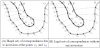
The main problem of the ICP is that is does not guarantee to produce a legal set of correspondences. By a legal set of correspondences is meant that there are no inversions between successive pairs of correspondences (see figure 3). In detail, when starting from a reference pair of corresponding points and traveling successive around the complete boundaries to pairs of correspondences, the arc path lengths in relation to the reference points always have to be increasing.
An extension of the classical Procrustes alignment to point-sets of differing point counts is known as the Softassign Procrustes Matching algorithm [8]. It alternates between solving for correspondence, the spatial mapping, and the Procrustes rescaling. The Softassign Procrustes Matching algorithm is also an iterative process and uses deterministic annealing to solve the optimization problem. In deed it is a very timeconsuming and computationally expensive procedure. They applied the algorithm to dense point sets not to closed boundaries. One-toone correspondences between points were established and points without correspondences are rejected as outlier. The establishment of point correspondences is only held in a nearest neighbor framework so they do not guarantee to produce legal sets of correspondences.
Another solution of the correspondence problem was presented by Belongie et al. [20]. He added to each point in the set a descriptor called shape context. The shape context of a point is a histogram which contains information about the relative distribution of all other points in the set. The histogram can provide invariance to translation, scale, and rotation. The cost of mapping two points is calculated by comparing their histograms using the χ2 test statistic. The χ2 distances between all possible pairs of points between the two shapes have to be calculated which results in a square distance matrix. The best match is found where the sum of distances between all matched histograms has reached its minimum. To solve this square assignment problem they applied a shortest augmenting path algorithm for bipartite graph matching which has a time complexity of O(n3). The result is a set of one-to-one correspondences between points with similar shape contexts. The algorithm can also handle point-sets with different point counts by integrating dummy points. But it is also not guaranteed that legal sets of correspondences were established.
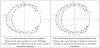
In none of these works is described the problem of aligning a convex to a concave shape. There arise special problems: Let us suppose that the concave shape representing the letter C is compared with the shape of the letter O (see figure 4). If the pair-wise correspondences were established between nearest neighbored points the resulting distance between both shape instances will be very small (see figure 4A). But intuitively we would say that these shapes are not very similar. In particular in such cases it is necessary to regard the order of point correspondences and to remove correspondences if they produce inversions. In addition to legality of correspondences it is important to take into account the complete contours of both shapes (see figure 4B). In result it can be seen that there arise big distances between corresponding points which leads to an increased distance measure.
4. Material Used for this Study
The materials we used for this study are fungal strains that are naturally 3-D objects but that are acquired in a 2-D image. These objects have a great variance in the appearance of the shape of the object because of their nature and the imaging constraints. Six fungal strains representing species with different spore types were used for the study. Figure 5 shows one of the acquired images for each analyzed fungal strain.
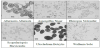
The strains were obtained from the fungal stock collection of the Institute of Microbiology, University of Jena / Germany and from the culture collection of JenaBios GmbH. All strains were cultured in Petri dishes on 2% malt extract agar (Merck) at 24°C in an incubation chamber for at least fourteen days. For microscopy fungal spores were scrapped off from the agar surface and placed on a microscopic slide in a drop of lactic acid. Naturally hyaline spores were additionally stained with lactophenol cotton blue (Merck). A database of images from the spores of these species was produced.
5. Acquisition of Shape Cases
5.1 Background
The acquisition of object shapes from real images is still an essential problem of image segmentation. For automated image segmentation often low-level methods, such as edge detection [8] and region growing [21,22] are used to extract the outline of objects from an image. Low-level methods yield good results if the objects have conspicuous boundaries and are not occluded. In the case of complex backgrounds and occluded or noisy objects, the shape acquisition may result in strong distorted and incorrect cases.
Therefore the acquisition is often performed manually at the cost of a very subjective, time-consuming procedure. In some studies it might be sufficient to reduce the shapes of objects to some characteristic points which are common features of the object class. Landmark coordinates [2,4,17,23] are manually assigned by an expert to some biologically or anatomically significant points of an organism. This has to be done for every single object separately. Additional landmarks can be automatic constructed using a combination of existing landmarks. The calculation of the position of these constructed landmarks has to by precisely defined, i.e. landmark C is located in the midpoint of the shortest line between landmark A and landmark B. Every single landmark is not only defined by its position but also by the specific and unique feature that it represents.
Landmarks might provide information about special features of an object contour but cannot capture the shape of an object because important characteristics might be lost. In many applications it is insufficient or impossible to describe the shape of an object only by landmarks. Then it is a common procedure to trace and capture the complete outlines of the objects in the images manually [14]. Indeed, manually image segmentation may be a very time-consuming and also inaccurate procedure. Therefore new semi-automatic approaches were developed [24,25] for interactive image segmentation. These approaches use live-wire segmentation algorithms which are based on a graph search to locate mathematically optimal boundaries in the image. If the user moves the mouse cursor in the proximity of an object edge, the labeled outline is automatically adjusted to the boundary. The manual acquisition of objects from real images with the help of semi-automatic segmentation approaches is faster and more precise.
As described in above we are actually studying the shape of airborne fungi strains. The great natural variance in the shape of these objects and the imaging constraints have the effect that a manual assignment of landmark coordinates is quite impossible. We also reject a fully automatic segmentation procedure because this might produce outlier shapes due to the objects might be touching and overlapping. Therefore we decided to use a manually labeling procedure in our application.
5.2 Acquisition of object contours from real images
As a shape we are considering the outline of an object but not the
appearance of the object inside the contour. Therefore we want to
elicit from the real image the object contour P represented by a set of
NP boundary points pk, k=1,2,...,Np. The user starts labeling the
shape of the object at an arbitrary pixel p1, of the contour P. In our
application we are only interested in the complete and closed outline
of the objects. So after having traced the object, the labeling should
end at a pixel pm, k=1,2,...,Np in the 8-neighbourhood of P1.
Because it might be difficult to exactly meet this pixel manually, the
contour will be closed automatic using the Bresenham [26] procedure.
This algorithm connects two pixels in a raster graphic with a digital
line. In addition to that we demand that two successive points may
not be defined by exactly the same point coordinates in the image. In
consequence we obtain an ordered, discrete, and closed sequence of
points where the Euclidean distance between two successive points is
either 1 or
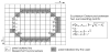
Figure 7 presents a screenshot from our developed program Case Acquisition and Case Mining - CACM while labeling a shape of the strain Ulocladium Botrytis with the point coordinates on the right side of the screenshot.
In fact image digitization and human imprecision always implies an error during the acquisition of the object shapes. It might be very difficult to exactly determine and meet every boundary pixel of an object when manually labeling the contour of an object. Also the quantization of a continuous image constitutes a reduction in resolution which causes considerable image distortion (Moiré effect). Furthermore the contour of an object in a digitized image may be blurred which means the contour is extended over a set of pixels with decreasing grey values.
5.3 Approximation
The amount of acquired contour points NP of a shape P depends on the resolution of the input image and on the area and the contour length of the object. To speed up the succeeding computation time of the following alignment process we introduced a polygonal approximation. The resulting number of points from a polygonal approximation of the shape will be influenced by the chosen order of the polygon and the allowed approximation error. We apply the approximation only to shapes which consist out of more than 200 points. This limit was introduced because the contour of very small objects in images might be defined by a few pixels only. A further reduction of information about the contour of these objects would be disadvantageous.
For the polygonal approximation, we used the approach based on the area/length ratio according to Wall and Daniellson [27] because it is a very fast and simple algorithm without time-consuming mathematic operations. Suppose the set of NP points p1,p2,...,pn, defining the contour of the object P, for which a polygonal approximation is desired. We use the first labeled point p1, as the starting point for the first approximation. Next we virtually draw a line segment from this starting point to the successor point in P. The area A between this line and the corresponding contour segment of P is measured. If the area A divided by the length of the line L is smaller then a predefined threshold T, then the same process is repeated for the next successor point in the set P (see Figure 8).
This procedure repeats until the ratio exceeds the threshold T. In that case the current point pm, becomes the end point of the approximated line and the starting point for the next approximation. The same process is then repeated until the first point p1, is reached. The result of the approximation is a subset of points of the contour P.
The ratio
5.4 Normalization of shape cases
In our application we demand the distance measure between two shapes to be invariant under translation, scale, and rotation. Thus, in a preprocessing step we remove differences in translation and we rescale the shapes so that the maximum distance of each point from the centroid of the shape will not be larger than one. The invariance to rotation will be calculated during the alignment process.
The centroid
To obtain invariance under translation we translate the shape so that its centroid is at the origin
Furthermore for each shape we calculate the scale factor tp:
This scale factor is applied to all points of the shape P to obtain the transformed shape instance P'. The set of acquired shapes are now superposed on the origin of a common coordinate system. The maximum Euclidean distance of a point to the origin of the coordinate system is one.
6. Shape Alignment and Distance Calculation
6.1 The alignment algorithm
In the Procrustes Distance (see Eq. 1) each of the shapes is rescaled in such a way that the standard deviation of all points to the centroid is identical (σP=σO). This normalization does not ensure that the resulting distance runs between 0 and 1. Since we are interested in comparing objects of different categories we rescale the shapes so that the maximum distance of a point to the centroid is not larger than 1. In comparison to Procrustes Distance we also do not need μP and μO because we have already removed the translation by transforming the objects into the origin.
The differences in rotation will be removed during our iterative alignment algorithm. In each iteration of this algorithm the first shape is rotated stepwise while the second shape is kept fixed. For every transformed point in the first shape we try to find a corresponding point on the second shape. Based on the distance between these corresponding points the alignment score is calculated for this specific iteration step. When the first shape is rotated once around its centroid, finally that rotation is selected and applied where the minimum alignment score was calculated.
We are regarding arbitrary shapes with varying orientations and different point counts and do not have any information about how the points of two shape instances have to be mapped onto each other. As already stated, we have to solve the correspondence problem before we are able to calculate the distance between two shape instances. In summary, for the establishment of point correspondences we demand the following facts:
- Produce only legal sets of correspondences,
- Produce one-to-one point correspondences,
- Determine points without a correspondence as outlier, and
- Produce a symmetric result, which is obtaining the same results when aligning instance P to instance O as when aligning instance O to P.
It was shown above that the establishment of legal sets of correspondences is an important fact to distinguish between concave and convex shapes. The drawback of this requirement is that the acquired shapes have to be ordered point-sets. The demand for establishing only legal sets of correspondences is also the main reason why we decided to extend the initial version of our alignment algorithm [28] that can only align concave with concave and convex with convex shapes. We extended our nearest neighbor-search algorithm presented there so that it can handle the correspondence problem while aligning concave with convex object shapes.
The input for our alignment algorithm is a pair of two normalized shapes P and O as described above. We define the shape instance P as the one which has less contour points then the second shape instance O. The instance with more points is always that one, which will be aligned to shape instance with less points. That means shape P will be kept fixed while shape O will be stepwise rotated to match P.
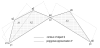
Before the iterative algorithm starts we define a range where to search for potential correspondences. This range is defined by a maximum deviation of the orientation according to the centroid (see Figure 9). This restriction will help us to produce legal sets of correspondences. The maximum permissible deviation of orientation γdev will be calculated in dependence of the amount of contour points nO of the shape O, which is the instance that has more points than the other one. Our investigations showed that the following formula leads to a well-sized range
The outline of our iterative alignment algorithm is as follows:

6.2 Calculation of point correspondences
The most difficult and time-consuming part is the establishment of point-correspondences. For each point pk with 1≤k≤np in the set P we try to establish exactly one corresponding point oj with 1≤j≤no in the set O. To create a list of potential correspondents we first select all points in O which are located in the permissible range of orientation (see Figure 9) and insert them into this list of potential correspondents {CorrList(pk)} of pk. Each of the selected points meets the following condition
with γpk the angle of point pk and γdev the permissible range of orientation around pk.
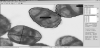
In Figure 10 is shown a part of two aligned shape instances at this state of registration. Each point in shape P is connected by lines to all of its potential correspondences. It can also be seen that there are outlier on shape O. As an outlier we define all points where no correspondence could be established. Resulting points without correspondences are a logical consequence if we demand one-to-one correspondences when mapping shapes with unequal number of points. Such kind of points does not have any influence on the calculated distance.
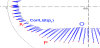
If no point in O is located in the permissible range {CorrList(pk)} is empty), pk is marked as an outlier. Normally in case of aligning convex objects there is no point in P which has not at least one potential correspondence. The permissible range of orientation is chosen big enough anyway. Indeed, this kind of outliers occurs only in cases of aligning convex to concave objects. Each point pk which has not a single potential corresponding point in O is included with the maximum distance of one when calculating the distance measure.
If there is at least one potential correspondent we calculate the squared Euclidean distances between pk and each point in this list. Then the points in this list {CorrList(pk)} were sorted with ascending distances in relation to pk. In succession we check for each point in this list if there was already assigned a corresponding point in P. The first found point without a correspondence is selected and we establish a one-to-one correspondence between them. If all points in the list {CorrList(pk)} have already a correspondence the point pk is marked as an outlier. In contrast to those outliers in P which do not even have one potential correspondence in O, this kind of outlier will not be included in calculating the distance measure.
Let us assume we had gone through the complete set P and assigned to each point pk either a correspondence in O or marked it as an outlier. In the next step we want to ensure to produce a legal set of correspondences. Therefore we go through the set P again and remove all one-to-one correspondences that are inversions (see figure 3). Suppose we have found a point pk assigned to a correspondence og in O that produces an inversion with the point pm which is assigned to the point of (k,m≤np; g,f≤no). First we try to remove the inversion by switching the correspondences, i.e. pk will be assigned to of and pm will be assigned to og. Otherwise we remove the correspondence of pk and check in succession all the remaining points in the list {CorrList(pk)} if it is possible to assign a correspondence with one of these points that does not produce an inversion. If we find a point in this list, we establish the one-to-one correspondence between these two points. Otherwise we have to mark pk as an outlier.
6.3 Calculation of the distance measure
The distance between two shapes P and O is calculated based on the sum of Euclidean distances. If there was assigned a correspondence to the point pk, 1≤k≤np in p, the Euclidean distance between this point and its corresponding point ok in O is calculated by
If the point pk is an outlier because there could not be assigned at least one potential correspondence and the list {CorrList(pk)} is empty, the distance is set with the maximal value of one
The sum of all pair-wise distances between two shapes P and O is defined by
Due to the fact that we interested in obtaining a distance measure which runs between zero and one, we normalize the sum according to nP, the number of points in P
The mean Euclidean distance alone is not a sufficiently satisfactory measure of distance. Particularly in cases of wavy or jagged contours important information get lost using the averaged distance. Therefore we also calculated the maximum distance between a pair of established correspondences
The final similarity measure is the weighted sum of the mean Euclidean distance and the maximum Euclidean distance
The choice of the value for the weights α and β depends on the importance the user wants to respective distance measure. We chose for α and β a value of 0.5 which results in an equal influence of both distances to the overall distance.
6.4 Evaluation of our alignment algorithm
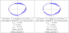
At first we will demonstrate that the algorithm is symmetric (see Figure 11), i.e. the same distance is calculated when aligning instance P to instance O as when aligning instance O to P. As described in above the instance with more contour points is always that one which will be aligned to shape instance with less points. Therefore, the order in which the cases are given as input into the algorithm doesn’t matter. A special case where the order matters is if both shape instances are defined by the same amount of contour points.
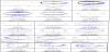
The following table presents some results of pair-wise aligned shape cases. In the left column of the table the visual results are shown with connecting lines between corresponding points. The right column of the table presents the calculated scores and the number of outlier which are included in the alignment score with a distance value of one. The alignment score of value zero means identity and the value of 0.5 can be understood as neutral. Up to a value of one the shapes become more and more dissimilar.
Again we take a closer look at the pair-wise alignment of a concave and a convex shape. Reconsider the example from above where the shape of the letter O has to be aligned to the shape of a letter C. Figure 13 presents a screenshot from our program where a similar situation occurred. There were twelve outlier determined on the convex shape which are included in the calculation of the alignment score. As more of these outliers are included as more dissimilar the two shapes become because each of them is assigned with the maximum distance of one.

Under these circumstances the points on the inside of the concave shape may not have any influence on the resulting alignment score. This is due to the fact that they were not mapped onto opposite points of the contour of the convex shape (see figure 4B). In deed, this is an error of the algorithm but otherwise it may happen that the alignment score exceeds the value one.
7. Conclusions
We have proposed a method for the acquisition of shape instances and our novel algorithm for aligning arbitrary 2D-shapes, represented by ordered point-sets of varying size. Our algorithm aligns two shapes under similarity transformation; differences in rotation, scale, and translation are removed. It establishes one-to-one correspondences between pairs of shapes and ensures that the found correspondences are symmetric and legal. The method detects outlier points and can handle some amount of noise. We have evaluated that the algorithm also works well if the aligned shapes are very different, like i.e. the alignment of concave and convex shapes. A distance measure which runs between 0 and 1 is returned as result.
The methods are implemented in the program CACM Version 1.4 which runs on a Windows PC.
Competing Interests
The author declare that there is no competing interests regarding the publication of this article.