


1. Introduction
Printed Circuit Board (PCB) is crucial part of electronic device it needs to be properly investigated before get launched. Automatic inspection systems are used for this purpose but due to more complexity in circuits, PCB inspections are now more problematic. This problem leads to new challenges in developing advanced automatic visual inspection systems for PCB.
Automatic Optical Inspection (AOI) has been commonly used to inspect defects in printed circuit board during the manufacturing process. An AOI system generally uses meth-ods which detects the defects by scanning the PCB board and analyzing it. AOI uses methods like Local Feature matching, image Skeletonization and morphological image comparison to detect defects and has been very successful in detecting defects in most of the cases but production problems like oxidation, dust, contamination and poor reflecting materials leads to most inevitable false alarms. To reduce the false alarms is the concern of this paper.
There are previous approaches for detecting defects of elec-tronic circuit board such as papers [1,2]. Maeda et al. [1] uses infrared light image to detect the defect by testing electrically, while Numada et al. [2] extracts the global features using the interest point and its surrounding points and detects the defect using Mahalanobis distance.
Papers for defect classification have been also proposed in papers [3] and [4]. Paper [3] improves the accuracy of classification using two images taken under the different Lighting conditions, and detects the defect region from the difference between the test image and the reference image which is prepared in advance. Support Vector Machine (SVM) [5] is used to classify into two classes of true defect and pseudo defect. Multiple classifiers are used with multiple subsets using random sampling of data set. The approach has an advantage to take voting processing for the defect classification when number of data set is large but it is still necessary to generate and prepare the reference image.
Paper [4] has been proposed as an approach without using reference image for the test of target defect. Key point extraction is used to crop the defect candidate region and SVM is used to classify the cropped defect region using the extracted features when cropped defectregion is input to the learned Convolutional Neural Network (CNN). However, this model is not applied to the multiple input images and it is not possible to make classification using two images taken under the different Lighting conditions.
In the computer vision fields such as image matching, channelwise concatenations of inputs or feature maps have been widely studied [6-8]. Research for classification of the flower image is also represented in the image classification [9]. This paper improves the accuracy by learning CNN using two images taken under the different lighting conditions. The proposed method tries to apply the multiple dimensional features originally under two different lighting conditions to the research field of defect classification of electronic board. No similar researches have been proposed in this defect classification field since the most previous researches of this defect classification of electronic board just use the feature vectors obtained from the original image and this paper tris to use two different lighting conditions simultaneously and develops the new contribution of this defect classification field using deep learning architecture. It is shown that the proposed approach improves the classification accuracy for the electronic board image with the defect through the comparison with the previous approaches. The effectiveness is also confirmed in the experimental results.
2. Materials and Methods
2.1 Lighting Conditions and Kinds of Defect
2.1.1 Lighting Conditions
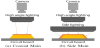
Test image used for this research is the detected defect by AOI, which was taken again by the device with the human eye check called “verification device”. Verification device takes two kinds of images under two different lighting conditions. Image taken with large angle lighting is named “coaxial main” and image taken with both side lighting and large angle lighting is named “side main” in this paper.
Figure 1 shows the outline of each lighting condition. Coaxial main and side main are ring lights structure and diameter of the side main is larger than that of coaxial main. Taking image with this structure enables not to make difference of position between two kinds of image. Coaxial main illuminates the board from the vertical direction as shown in Figure 1(a) while side main illuminates board from side directions in addition to the vertical direction as shown in Figure 1(b).
2.1.2 Kinds of defect
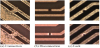
Defects of the electronic board consists of true defect and pseudo defect. True defect cannot be used as a product and it is necessary toremove the true defect at the checking test, while pseudo defect is no problem to be used as a product by removing the dust and so on. True and pseudo defects are classified into several kinds based on the color and shape. Same kind of defects have different features in an image and this may cause difficult classification problem.
Images of true defects in the electronic board are shown in Figure 2, Similarly images of pseudo defects in the electronic board are shown in Figure 3. Upper images are taken by thecoaxial main lighting conditions and lower images are taken by the side main lighting conditions. Coaxial main lighting is useful to the attached foreign matter, color change, and lack and so on, while side main lighting is useful to the edge, 3D defect, projection, and foreign matter.
2.2 Multi-Input CNN model
Deep learning and CNN technologies have been introduced as the effective pattern recognition approach in computer vision. CNN has been high contributions since AlexNet [10] (2012) in the ImageNet Large Scale Visual Recognition Challenge (ILSVRC) [11]. CNN mainly consists of convolutional layers, pooling layers and full connected layers. Convolutional layers and pooling layers are important since convolutional layers calculate convolution of image and multiple filters, extract the features where abstraction features are obtained in the deeper layer. While pooling layers shrinks the size of output map from the convolutional layer and prevents the overfitting.
Proposed approach classifies into two classes of true defect or pseudo defect by inputting two images under the coaxial main lighting image and the side main lighting image. This paper considers two multi-input CNN for the performance of classification accuracy. The first one is the CNN which is connected at around the output layer after connecting the one dimensional vectors with convolution and pooling three times respectively to each input image. The second one is the CNN which is connected at around the input layer after connecting vectors with processing convolution and pooling one time respectively to each input image.
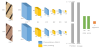
2.2.1 CNN Architecture Connecting at around Output Layer
CNN architecture which connects at around output layer is shown in Figure 4. All convolution layers C1 consist of 32 kernels of size 4 and slide side is 1. Pooling layer S1-2 consist of pool size 3 × 3. Pooling layer S3 consists of pool size 2 × 2 and the same size of slide. Drop out is applied to the output which connected the output of S3 with smoothing. Fully connection layers FC1-2 have 64 neurons respectively. Sigmoid function is used as activation function of output layer.
2.2.2 CNN Architecture Connecting at around Input Layer
CNN architecture which connects at around input layer is shown in Figure 5. All convolution layers C1 consist of 32 kernels of size 4 and slide size is 1. Pooling layer S1consist of pool size 3 × 3. Output of pooling layer is connected to one.
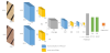
Convolution layer C3-4 consists of 32 kernels of size 4 and the slide size is 1. Pooling layer S2-3 consist of pool size 3 ×3. Drop out is applied to the output which connected the output of S3 with smoothing. Fully connection layers FC1-2 have 64 neurons respectively. Sigmoid function is used as activation function of output layer.
3. Results and Discussion
3.1 Dataset and data augmentation
Data set consists of 805 samples respectively for coaxial main lighting and side main lighting image with 256 × 256 pixels. Numbers of true defect and pseudo defect are 470 and 335 respectively. 50 samples of true defect and 50 samples of pseudo defect are randomly selected for the testing evaluation and remained 420 true defects and 285 pseudo defects are used for the learning.
From the situation that number of learning data is not enough for the sufficient learning, data augmentation is applied and number of learning images were increased to 5 times of the original data with flip horizontal, rotation and scaling transformations.
3.2 Experiments
Two Multi-inputs CNN were used for the learning by inputting actual electronic circuit board images. Keras [12] was introduced as a high level neural network library for the implementation. Binary cross entropy was used for the loss function and SGD and Adam [13] were used for the optimization. Initial value for the learning rate was 5e-4 and momentum parameter was 0.9 and parameter to decreasing of learning rate at each epoch was 1e-4 as parameters of SGD. Learning rate was lr=5e-4 and parameter to decreasing of learning rate at each epoch was 1e-4 as parameters of Adam. Other parameters were given in the similar way as β1 = 0.9, β2 = 0.999.
Let the learning rate of Adam be lr, initial learning rate be lr0, parameter to decreasing at each epoch be k, number of epoch be t, then learning rate is updated using Equation (1).
lr = lr 0/(1 + kt)
Learning was done under the condition of batch size 32 and maximum epoch 100. Table 1 shows the confusion matrix when positive sample means true defect while negative sample means pseudo defect.
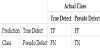
Table 2 shows the classification results. Here let the CNN connected at around output layer be CNN1 and the CNN connected at around input layer be CNN2.
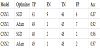
Table 2 suggests that CNN2 gives the higher accuracy than CNN1 using both optimization algorithm. It is suggested that CNN connected at around input layer can learn the better features from the property that position does not change between both lighting conditions. It is also confirmed that CNN2 gives the same level accuracy in both optimization algorithms but CNN1 suggests Adam gives better accuracy than SGD.
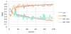
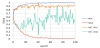
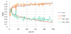
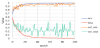
Figure 6-9 show the transitions of Accuracy and Loss for each condition. Blue line represents "Training Accuracy", red line represents ”Training Loss”, orange line represents "Validation Accuracy" and green line represents "Validation Loss", respectively. Figure 6-9 suggests Adam gives faster optimization in the learning than SGD in any Multi-input CNN.
3.3 Comparative experiments
Proposed approach was compared with two previous classification approaches. One is to use SVM for the classification after using a learned CNN as feature extractor as shown in paper [4]. The other is Fine-tuning of learned CNN using small number of data set. ImageNet [14] was learned to VGG16 [15] and this CNN model used for the feature extraction and finetuning.
CNN features were extracted as 4096 dimensional features from fc7 layer of learned VGG 16 of ImageNet. Then extracted features were learned by linear SVM. Three cases of learning CNN features by SVM are evaluated for the cases of using only the coaxial main, only the side main and using both of them. When two lighting images are used for the classification, 4096 dimensional features are extracted, connected and 8192 dimensional features were used. Classification results are shown in Table 3 using the extracted CNN features and SVM.
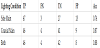
Table 3 suggest that using both lighting condition gives best classification accuracy.
In the fine-tuning of VGG16 which learned ImageNet, size of input layer was changed to (256,256,3), number of output layer was changed to 2 from the original 1024. Binary cross entropy was used as loss function and SDM and Adam [13] were used for the optimization.
Initial value for the learning rate was 1e-4 and momentum parameter was 0.9 and parameter to decreasing of learning rate at each epoch was 1e-4 as parameters of SGD. Learning rate was lr=1e-4 and parameter to decreasing of learning rate at each epoch was 1e-4 as parameters of Adam. Other parameters were given in the similar way as β1= 0.9, β2= 0.999. Learning rate is updated using Equation (1). Learning was done under the condition of batch size 32 and maximum epoch 100. Table 2 shows the classification results. Classification result of fine-tuning of VGG16 which learned ImageNet is shown in Table 4.

Accuracy Graph of comparison with CNN1, CNN2, CNN feature and SVM, Fine-tuning of Learned CNN is shown in Figure 10. Finetuning1 represents the learned result of coaxial main images, while Fine-tuning 2 represents the learned result of side main images. CNN Feature + SVM represents the result using both coaxial main and side main images. CNN1, CNN2, Fine-tuning represent the accuracy for he learned CNN using Adam optimization algorithm.
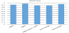
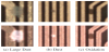
Figure 10 suggests that CNN2 connected at around input layer gives the best accuracy and Fine-tuning 2 (of VGG16 learned for ImageNet) gives the second best accuracy. It is also confirmed that side main lighting images gives better accuracy than coaxial main images from Table 3 and Figure 10. These results suggest that CNN2 gives the higher classification accuracy by learning the features between two different lighting images at around input layer. Some misclassified images by Fine-tuning 2 but correctly classified images by CNN2 are shown in Figure 11. Upper images are side main images while lower images are coaxial main images.
Fine-tuning 2 misclassified the image which were difficult to see the defect position by the coaxial main lighting but CNN2 using both images could correctly classify the defects in Figure 11.
4. Conclusion
This paper proposed a new approach using multi-input CNN architecture to use two different lighting images and evaluated the classification performance using defect images of electronic circuit board. Previous approaches need the reference images under two lighting conditions, while the proposed approach does not need reference images and could correspond to the defect classification using CNN from the feature extraction and classification process.
The evaluation in the experiments suggest that CNN connected at around input layer gives the highest accuracy in defect classification via comparison with two different CNN architectures. Further the proposed approach was compared with the CNN feature + SVM, and Fine-tuning from the learned CNN. It is shown that the proposed Multi-input CNN2 gave the best classification accuracy among them.
True defects consist of connection, projection and lack while pseudo defects consist of large dust, dust and oxidation. Classification was performed to the true and pseudo defect but classifications into multiple cases or corresponding to the multiple defects in an image are remained as future works.
Competing Interests
The authors declare that they have no competing interests.
Acknowledgments
Iwahori’s research is supported by JSPS Grant-in-Aid for Scientific Research (C) (17K00252) and Chubu University Grant.