2.1 Problem statement

A NoC-based architecture consists of a set of interconnected Intellectual Property (IP) components. Such IPs are typically general purpose or specific processors, dedicated hardware accelerators, and peripheral controllers or memories in a single chip. They are emitters and/or receivers of messages. The components are connected by routers according to a given network topology. Each IP is associated with a unique a router through its network interface (NI). More formally, a NoC can be modeled by a directed graph G = (V,A), where the set V of vertices represents the routers and IPs, and the set of arcs A ⊆ V ×V represents the directed transmission links between them. Here, we consider wormhole routing. Each message μ is made of a sequence of l(μ) contiguous packets, with |l(μ)| = lμ > 0, that are transmitted along the arcs of the network. The header packet contains a specification of the message origin/destination path, while other packets are application-dependent data. A router has no memorization capacity, it only retransmits packets as specified by the header packet. The NoC is synchronous, it is cadenced by a common clock shared by all its components. Each arc has a capacity of 1 packet by unit of time, called a time-slot or time-step. The packets are transmitted in a contiguous way. Hence, if a physical occurrence of a message emitted at time t(μ) follows the path i, i+1, . . . , i+n, with i Є V, its packets will cross the arc (i, i+1) at the consecutive timesteps t(μ)+i+q,q = 0, . . . , l_μ −1. We say that an arc may be “occupied” by a packet at a given time-slot, otherwise it is said “free” at a given time-slot.

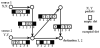
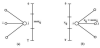
To guarantee transfer rate, a source repeatedly emits messages based on a period or cycle T. A given bandwidth is specified by a message size, i.e., the number of packets emitted by period T. Hence, a message can be seen as a class of its physical occurrences at each cycle. This allows to consider classes of time-slots for arc occupations. If an arc is occupied at time-slot t, it will also be occupied at timeslots t +λT, for all nonnegative integer λ. We say that an arc is occupied at t modulo T to express its recurrent occupation by a packet. We will often talk of a packet, or message, to refer to the class it represents. When transmitted through the network, two packets are said conflict-free if they never clash, i.e., cross an arc at the same time-slot. By extension, paths or messages are said “conflict-free” or “contention-free” when their related packets never conflict (two at a time). Since paths may share common communication links, and since we want to achieve guaranteed traffic, paths and emission dates have to be stated such that two packets will never clash. We assume that paths may contain circuits, only when those circuits do not contain the destination or the origin of the path. Indeed, if the origin appears in a circuit, then the message can be send later without that circuit, and if the destination appears in a circuit, then all the corresponding traffic is useless and can be removed. However, a circuit that does not involve the destination nor the origin may be useful to wait for a region of the network to be less heavily loaded. Figure 1 illustrates two conflict-free source/ destination paths in an already occupied NoC, with an emission cycle of length T = 5. Two packets are emitted from source 1, and two packets from source 2. A table of the available time-slots (modulo T) that packets can use as they advance through the network is shown next to each arc, and filled squares are unavailable time-slots. We can see that packets cross the shared arcs at distinct time-slots modulo T and never conflict. We can now precisely state the combinatorial optimization problem called “Cyclic K-conflict-free shortest Paths Problem” that we address in this paper.

Figure 1: Two message transfers in an occupied NoC.

2.2 Cyclic K-conflict-free shortest Paths Problem (CKPP)

A problem instance consists in a directed graph G = (V,A), an emission cycle of length T, and a set of K messages defined by

M={ μ k =( s k , d k , l k ): s k ∈V, d k ∈V, l k >V,k=1,...,K}

where (s_k,d_k) is an origin/destination pair, and lk the number of packets of the message. The goal is to find the departure times of the messages t(μ_k) Є [0,T −1], μ_k Є M, at each source node and the origin/destination paths of minimum total length for conveying the messages, such that the paths are conflict-free.

We should note that the objective of the problem is the total length of the paths, whereas the constraints reside in the temporal occupation of the arcs such that paths are conflict-free. It is worth noting that the problem is NP-hard in the strong sense for general graphs as well as for planar graphs or grid networks. This can be seen by relating the problem to the K-Edge-Disjoint Shortest Paths problem (EDP) [16]. This well known problem has different versions depending whether we ask for vertex or edge disjoint paths between a set of K source-sink pairs. This is one of Karp’s [17] original NP-hard problems. By restricting CKPP to only those instances for which T = 1, we retrieve the EDP. This problem is known to be NP-hard in the case of planar graphs [18], even when stated in the grid and when path lengths are constrained by a constant [19]. Then, since CKPP remains NP-hard when the number T is bounded by a constant, it follows that it is NP- hard in the strong sense. Similarly, the CKPP can be seen as an extension of a Bin Packing problem, where arcs stand for bins of capacity T, and the K messages for items of size q_k.

A similar problem is the unsplittable flow problem (UFP). It is a generalization of EDP where every edge e has a positive capacity c_e; and every pair has a demand f_k > 0. The demand from s_k to d_k has to be routed in an unsplittable manner, i.e., along a single path from s_k to d_k. For every edge e the total demand routed through that edge should be at most c_e. The problem adds a capacity constraint to the EDP. It is different from CKPP since it allows variable arc capacities, discarding temporal aspects on arc occupation. Generally, classical flow models only deal with static situation. A well-known problem that introduces time dependent transit constraints is the one-to-one shortest path problem with time windows (SPPTW) [20]. The aim is to compute a shortest path respecting the given time-windows on arcs occupation. This kind of problems often arises in terrestrial transportation, road traffic control, and vehicle routing applications. An example is Automated Guided Vehicles (AGVs) [21] technology for optimizing large scale production and logistic systems. The SPPTW is NP-hard but several pseudo-polynomial time algorithms are available to solve it exactly [20,22,23]. A sub-problem of our CKPP is to compute a one-to-one source-destination path in an already occupied NoC. The available (“free”) time-slots on each arc stand for time-windows. Hence, a modified Dijkstra algorithm can be designed to compute such a single path in an efficient way. It will be used as an operator into the heuristic methods presented in this paper to address the whole CKPP.

2.3 Time-expanded graph approach

We address the problem by using a spatiotemporal graph as a memory of temporal arc occupation. This memory specifies for each arc of the network, and each time-slot in interval [0,T −1], whether or not the arc is occupied by a given packet at the given time slot. We say that an arc is “free” or “occupied” at time t modulo T. Hence, an array of booleans of size T is associated to each arc. Such a spatiotemporal graph is generally called a time-expanded graph (TEG)[15]. In its standard definition, a TEG contains one copy of the node set for each discrete time step. This is a time layer. For each arc in the original graph, there is an arc copy between each pair of time layers in the TEG. When time occupation is cyclic, as in our case, each layer t is connected to its next (t +1) modulo T layer. The notion was presented by Ford and Fulkerson [24] in order to model flow over time. The memory size needed is O(N² ×T) for general graphs or O(N × T) for planar graphs, with N the number of nodes. As reviewed by K¨ohler et al. [15], the TEG concept allows to solve a variety of flow-overtime problems by applying algorithmic techniques developed for static network flows. It is worth noting that the size of the timeexpanded network is only pseudo-polynomial in the input size, since the number T is encoded with log(T) bits. Hence, we should address only instances of moderate size T. Fortunately, since T is always small (maximum of 47 time-slots in our applications), the TEG approach is a natural way to deal with shortest path findings that would guarantee traffic in a NoC.

2.4 Mixed integer linear programming model

We first propose an ILP of the CKPP. The model is packet oriented. A NoC is composed of a set ℐ of IPs ( |ℐ|=P ) and a set ℛ of routers ( |ℛ|=N ) . A set ℘ of packets ( |℘|=Q ) with a specific origin and destination (taken from ℐ ) has to travel across the NoC without conflicts and in the shortest possible time. The set of IPs and routers form the nodes of the graph V ={0, . . . ,P−1,P, . . . ,P+N−1}. The set of arcs is denoted by A ⊆ V×V. There are |Q| packets indexed by q, q Є {1, . . . ,Q} such that where l_k is the size of message as stated in the CKPP definition. Each packet q starts and ends in an IP, i.e. has an origin s_q in ⊆ , s_q Є {0, . . . , P−1} and a destination d_q in ⊆ , d_q Є {0, . . . , P−1} with s_q ≠ d_q. Time is discretized, t Є {0, . . . ,T −1} is a time slot, and T is the TDMA size. The system is pipeline-based, thus, time slots t and t +T are identical for all t. Let x_i,j,q,t be a boolean variable set to 1 if packet q uses arc (i, j) during time slot t, 0 otherwise. With the previous definition, we can state the constraints and the objective function as a 0-1 integer linear program in Equations (1-11) below.

1. Arc capacity: Each arc is used for conveying at most one packet per unit of time.

   ∑ q∈{1,...,q} x i,j,q,t ≤∀(i,j)∈A,∀t∈{0,...,T−1} (1)

2. Packet origin: For all q Є {1, . . . ,Q}, packet q originates from IP s_q Є {0, . . . ,P−1}.

   ∑ t∈{0,...,T−1} ∑ j∈{P,...,P+N−1}         |( s q,j )∈A x s q ,j,q,t =1  ∀ q ∈{1,...,Q} (2)

3. Packet destination: For all q Є {1, . . . ,Q}, packet q has to reach IP d_q Є {0, . . . , P−1}.

   ∑ t∈{0,...,T−1} ∑ i∈{P,...,P+N−1}         |(i, d q )∈A x i , d q ,q,t =1  ∀ q ∈{1,...,Q} (3)

4. Packets conservation: For all instant time t Є {0, . . . ,T −1}, for all q Є {1, . . . ,Q} and for all i Є {P, . . . ,P+N −1}, if packet q reaches router i at time t, then it has to leave that router at time t +1.

   ∑ j∈V|(j.i)∈A x j,i,q,t ∑ i∈V|(i,j)∈A x j,i,q,(t +1) mod T ∀t∈{0,...,T−1}, ∀q∈{1,...,Q} ∀i∈{P,...,P+N−1} (4)

5. Origin IPs are not reentrant: For all instant time t Є {0, . . . ,T −1}, for all q Є {1, . . . ,Q}, packet q cannot enter IP s_q Є {0, . . . ,P−1}.

   ∑ i∈(P,...,P+N−1)|(i, s q ) x i, s q ,q,t =0  ∀t∈{0,...,T−1}, ∀q∈{1,...,Q} (5)

6. Destination IPs are not reentrant: For all slot time t Є {0, . . . ,T −1}, for all q Є {1, . . . ,Q}, packet q cannot leave IP d_q Є {0, . . . ,P−1}.

   ∑ j∈(P,...,P+N−1)|( d q ,j)∈A   ∀t∈{0,...,T−1}, ∀q∈{1,...,Q} (6)

7. Origin IPs generate at most one packet at a time: For all time slot t Є {0, . . . ,T −1}, for all IP i Є {0, . . . ,P−1}, the sum of the packets q sent out of i and such that sq = i must be less than one.

   ∑ q∈{1,...,Q} | s q =i ∑ j∈{P,...,P+N−1} |(i,j)∈A   x i,j,q,t ≤1 ∀t∈{0,...,T−1}, ∀i∈{1,...,P−1} (7)

8. Destination IPs consume at most one packet at a time: For all time slot t Є {0, . . . ,T −1}, for all IP j Є {0, . . . ,P−1}, the sum of the packets q sent to IP j and such that dq = j must be less than one.

   ∑ q∈{1,...,Q}   | d p =i ∑ i∈{P,P+N−1}         |(i,j)∈A x i,j,q,t ≤1   ∀t∈{0,...,T−1}, ∀i∈{P,...,p+N−1} (8)

9. Message constraints: A message is modeled as a sequence of packets that must have the same route in the NoC. More formally, message k Є {1, . . . ,K} is an ordered set of packets {ω_k,1, . . . ,ω_k,l(k)} where l(k) is the length of message k (i.e., the number of packets in the message). ω_k,1 Є {1, . . . ,Q} is the first packet and ω_k,l(k) is the last packet of message k. In any consistent instance, all the packets of a message must have the same origin and destination router, i.e., they must satisfy: s_q = s_q' and d_q = d_q' ∀k∈{1,...,K}, ∀ q,q' ∈{ ω k,1 ,..., ω k,l(k) } The message constraints are enforced as follows: x i,j, ω k ,q, t = x i,j, ω k ,q+1 , (t+1)modT ∀k∈{1,...,K},   ∀q∈{1,...l(k)−1} ∀t∈{0,...,T−1}, ∀(i,j)∈A , (9) These constraints say that if packet wk,q occupies arc (i, j) at time t, then packet ωk,q+1 must occupy this arc at time (t+1) mod T. The equality also enforces that if packet ω_k,q does not occupy arc _{(i, j)} at time t, then packet ω_k,q+1 cannot occupy this arc at time (t +1) mod T. Thus, all the packets of a message move along the same route within a time shift.
10. Packet destination: The destination d_q of packet q is a terminal node of the path of the packet q. For all time slot t Є {0, . . . ,T −1}, for all q Є {1, . . . ,Q}, the packet q cannot go to another destination other than its destination d_q.

    ∑ j∈{0,...P−1}−{ d q }           (i,j)∈A x i,j,q,t ∀t∈{0,...,T−1},   ∀q∈{1,...Q} ∀i∈{P,...,N+P−1}, , (10)

11. Objective: Minimize the total length of all paths for all packets

    Min ∑ (i,j)∈A ∑ q∈Q ∑ t∈T x i,j,q,t (11)

When compared with the CKPP problem definition which is a slightly more general formulation, Constraints 7 and 8 are specifically added to take into account the hardware conditions of emission and reception. These conditions state that each IP node implements a TDMA (Time Division Multiple Access) table that can only send one single packet at each time slot occurrence. A router node, at the difference of an IP node, allows packets to cross at a given time slot following the different directions stated by the communication graph. An IP node will always be connected to a single router and its emission capability restricted by the TDMA mechanism such that no more than one packet will be emitted or received at each time slot.

3.1 Iterated local search main loop

We choose one of the simplest ways to address the problem by means of heuristic methods, that is, by a simple iterated local search scheme that exploits randomized choices [25]. The main loop simply iterates a search many times by restarting the algorithm from a new random starting point. We identify two levels of operations. The first level puts the emphasis on the fast construction of partial solutions. It manages the message emission dates and then, applies a set of construction operators. Starting from such a solution, the second level applies local modifications on the path set in order to “improve” or “repair” the solution. Improvement is based on a neighborhood operator that explores a smaller region around the current solution. The construction search is followed by an improvement search as often in heuristic methods. Hence, the iterated approach respectively, alternates large and small moves in the search space. Large construction moves are for diversity generation, whereas small improvement moves for intensification of the search in a particular region. The pseudo-code of the main loop is presented in Algorithm 1. The two internal calls “constructSolution” and “improveSolution” respectively correspond to the construction trial followed by the improvement trial. These two procedures are detailed in the next sections. In each case, possibly non admissible solutions can be generated. That is why solutions must be ranked according to the hierarchical two objectives of respectively the number of built paths and the paths length. Maximizing the number of built paths is the first objective, whereas minimizing the paths length is the second objective. The “selectBest” procedure performs such a ranking.

3.2 Construction loop

Here, we present the structure of the construction procedure referred to as constructSolution in the main loop of Algorithm 1. The procedure is detailed in Algorithm 2. Its role is to quickly generate new candidate solutions, admissible or not, that present the maximum number of paths built. To do so, the procedure iterates a basic construction process maxConstruct times. The first type of operations is the management of the message departure dates. Once the emission dates are set, a greedy parallel construction operator tries to quickly and simultaneously generate the K conflict-free paths. Then, a modified Dijkstra algorithm, which is more time consuming, only tries to rebuild the residual “blocked” paths one by one. The selectBest procedure performs a ranking as explained in the previous section. The main operators are detailed below.

Emission date management. As mentioned in the problem definition, the construction of admissible source/target paths mainly depends on the message emission dates that are specified in each

TDMA table of each source node in the interval [0,T −1]. Assuming that the emission dates are first set at initialization, it is necessary to make evolve such dates while constructions are reiterated. Two operators are proposed in order to manage emission dates. They are respectively named permuteDepartureDates and translateDepartureDates in Algorithm 2. The first operator is applied with probability 0.5. In each operator, a given TDMA table (i.e., a source node) is first chosen randomly. The first operator applies a random permutation between two emission dates of that TDMA table. The second operator applies a one time unit forward translation to the TDMA emission dates.

Greedy parallel construction. This procedure, called constructSolutionPar in Algorithm 2, greedily builds the origin/destination paths step by step and in a parallel way. Before this procedure can proceed, a set of routing tables must first be computed at the whole initialization. They embed the costs of the shortest paths from each location to all destination nodes in the original NoC graph. These tables are computed only once at the initialization of the main algorithm. The origin/destination paths are built step by step, i.e., time slot by time slot, and jointly. An image of the behavior of the algorithm is that of several waves that propagate in all directions at constant speed, from the source node until it reaches the destination node or not. Each iteration step corresponds to a given time-slot, and to the introduction of the next vertex into each path. The next router is chosen according to the minimization of its distance to the destination node, and by verifying in the TEG that the corresponding arc is free for the message packets. When several choices are available, the next vertex is chosen randomly. Then, the arc status structure is updated in the TEG. The process continues until all messages have reached their destination node, or no vertex insertion is possible. Then, a path is said “constructed” or “blocked”. The temporal complexity is O(N ×T²) for planar graphs, or graphs with constant degree, and O(N²×T²) for general graphs, with N the number of nodes and T the emission cycle. This is a rough estimation. A node can be visited as soon as there is an available time-slot in some incident arc, then it can be visited at most O(N ×T) for general graphs and messages of size 1. The number of time-slot examinations at each node depends on the degree of the node and message size, then it is at most O(N ×T) for general graphs and a message of size T.

Dijkstra algorithm in TEG. We have designed a breath-first-search algorithm able to construct a one-to-one shortest path in an occupied time-expanded graph. Here, the TEG may contain “free” or “occupied” arcs as part of the input. The procedure is called constructSolution WithModifiedDijkstra in Algorithm 2. The term Dijkstra is used in reference to the function of the algorithm, that produces a shorter path, and to the fact that it is a simplification of the classical Dijkstra algorithm with unit costs associated to the arcs. The algorithm is extended to take into account the cyclic nature of the problem and multi-packet traveling. Each iteration of the algorithm corresponds to a single time-slot increment, so that the path length increases of one time-unit. Thus, all the successors of a visited node are necessarily in minimum distance from the origin and will constitute the nodes to visit in the next iteration. A main simplification over the classical Dijkstra, is that we do not have to manage an unordered list of successors and select lower cost one. All successors are at lower cost necessarily and must be examined. As well as in Dijkstra’s algorithm, multiple predecessor node choices are possible. In this case, only one of the possible predecessors is selected randomly. Then, only one single path is computed based on these random choices since the embedding metaheuristic only necessitates one random single path at each call of the Dijkstra algorithm. Randomness must allow diversity of the paths found due to multiple calls. The temporal complexity is O(N ×T²) for planar graphs, and O(N²×T²) for general graphs. A node of the communication graph cannot be visited more than T times, otherwise the visit will constitute a loop in the TEG where nodes are duplicated T times. The number of time-slot examinations at each node depends on the graph degree and message size, then, it is at most O(N×T) for general graphs and a message of size T.

Another important difference with a standard Dijkstra algorithm arises from the cyclic and multipacket nature of the shorter path problem. Here, arcs occupation must be dynamically updated into the TEG as the path is currently built. This is necessary in order to avoid self-conflicts for a given multi-packet message, since a header packet could hit queue packets at the same emission cycle or at different emission cycles. The situation can occur if the length of a path is larger than the period T, but it can also occur with a message with length sufficiently large such that the header packet could hit its queue packets according to a loop in the path, regarding the NoC communication graph. This dynamic change of TEG occupation status has a direct impact on the conditions of optimality. In the case of a single packet message, the algorithm guarantees optimality in time polynomial with the TEG size, that is, in pseudo-polynomial time over the CKPP instance size. This naturally follows from the breath-first- search algorithm behavior. However, in the case of a multi-packet message and due to dynamic updates of arc occupation, optimality is no longer guaranteed. It arises that further arc/vertex choices should depend on the previous choices made. This is an indication of a more complex and specific problem. We actually do not prove some NPhardness for that specific subproblem, nor prove that a polynomial solution exist. At the moment of writing, we let the complexity analysis of that specific subproblem open. However, the less the number of packets, the more the probability to get an optimal one-to-one path. The shorter will be the path, the less will be the probability of conflict. Some possible solution that could be envisaged to guaranty optimality could be to delegate the single shorter path computation to the ILP method, once adapted to a given occupied TEG as an input. This could be envisaged in further work that would combine exact and heuristic methods.

3.3 Local search improvement algorithms

We now detail the improvement procedure, called improveSolution in Algorithm 1. While the construction procedure generates diversified solutions starting from random initializations, the improvement procedure allows to perform more or less smaller steps in a smallest region of the solution space in order to transform non admissible solutions to admissible ones. The general scheme of an improvement procedure consists of embedding a neighborhood operator within some search strategies. We first detail the neighborhood operator, then we propose three versions for the search strategy.

The pseudo-code of the neighborhood operator, called generate- Neighbor, is given in Algorithm 3. Because of the many paths constructions that need to be performed, we choose to operate at the level of paths deconstruction and reconstruction. The neighborhood operator simply suppresses a subset of the solution paths, with the removeMessages procedure, and hence tries to construct the solution again from that partial solution. To do so, it uses the greedy parallel construction procedure followed by the one-to-one Dijkstra algorithm, that were specified for the construction phase (cf. previous section). The number of removed paths stands for the neighborhood size, that can be more or less large. It is intended that the new paths, together with the previously “blocked” paths, would have a new chance to being completely reconstructed by the operator. Since many random choices are possible during path construction, the neighborhood can be seen as large, and the method interpreted as a “reparation” procedure, following the ruin and recreate principle as formulated by Schrimpf et al. [26].

Three versions of a search strategy are considered that embed the neighborhood operator. They are respectively a basic random walk search, that we call iterated random search (IRS), as specified in the pseudo-code of Algorithm 4, and two local search schemes, that are, a greedy descent local search, also called first improvement local search (ILS-FI), specified in Algorithm 5, and a steepest descent local search, also called best improvement local search (ILS-BI), specified in Algorithm 6. The iterated random search simply makes evolve the current solution by performing a given number of successive neighborhood moves, and then selects the best solution encountered. The method is very simple since very few operations are performed at each iteration step. This can be seen on Algorithm 4. On the contrary, the two local search schemes involve two internal loops each. As shown in Algorithms 5 and 6, the outer loop controls the depth of the search. The algorithms stop when no improvement has been found. Because all algorithms are random, there is no guarantee that a local minimum has been reached even if the algorithm does not make any progress. A given solution constitutes the pivot element around which are performed the neighborhood search. Hence, the inner loop, that is the difference between Algorithms 5 and 6, deals with the pivoting rule, that determines to which better neighboring solution to move to. When compared to the iterated random search above, note that a supplementary variable S' has to be added to allow testing the improvement move. In the greedy descent local search version, the first encountered best solution becomes the new pivot element. In the steepest descent version, it is the best solution within the whole neighborhood that must be selected as the new pivot element. Here, since the neighborhood is large and the method stochastic, the procedure only examines a random sample of the neighborhood set. The sample size is represented by the neighborhoodSampleSize parameter in Algorithms 5 and 6. In experiments, it is set to 100 neighbors to examine. Another important parameter is the neighborhood size itself, which is the maximum number of paths selected for suppression in a single neighborhood move. Its impact on performances will be investigated in experiments. It is set to a maximum of nbMsg paths suppressed, with K being the total message number. This means that at each move, the exact number of suppressions is chosen randomly between 1 and K paths. Note that this parameter is shared by both IRS and ILS methods.

4.1 Impact of the main algorithmic components

In this section, we study the performance of different combinations of the construction/improvement operators and of the Dijkstra procedure. We use the iterated random search (IRS) method specified by Algorithm 1, in which the construction method constructSolution corresponds to Algorithm 2 and the improvement method improveSolution corresponds to Algorithm 4 to perform the experiments. Adding or not the Dijkstra component, we study the impact of construction and improvement operations when adjusting the maxCount, maxConstruct, and maxImprove algorithm parameters. The goal is to illustrate the importance of each added new algorithm component that improves both computation time and quality of solution substantially at the same time. The algorithm stops once an admissible solution is found or when the maximum number of iterations is reached.

Results are reported in Table 1. The procedure was executed on the N3A(9-15-10-27) instance of Figure 8, for four different combinations of the IRS loops. Results are averaged over 100 runs. Since it may be the case that no admissible solution is produced during a run, we report in a column named “Paths built”, the average percentage of built paths related to the message number. We also report the average computation time in seconds in the column named “CPU time”, and the number of feasible solutions obtained over the 100 runs in column “Feas. sol.”. Numerical results are given within six rows for construction phase only, with construction respectively iterated 1, 1000, and 100000 times. For each configuration of the iteration number, results are reported with or without the Dijkstra component. The last configuration corresponds to the introduction of the improvement loop and reiteration of the construction/improvement phase. For this experiment, the algorithm parameters (maxCount,m axConstruct,maxImprove) will take the values (50, 1000, 1000). The outer loop reiterates 50 times the construction/improvement phases, each one executing 1000 internal iterations.

Table 1: Impact of the main algorithmic components on N3A instance.

4.2 Comparative evaluation on the real-life benchmark set

We now compare the different approaches considered in this paper, including the ILP solution, on the five real-life benchmarks. We also evaluate solutions for three different values of the neighborhood size. The three heuristics are specified in Algorithms 1-6 with their default parameters. In the iterated random search (IRS) method, the combination of construction/improvement operations are set to the values (maxCount,maxConstruct,maxImprove) = (50,1000,1000). In the iterated local search (ILS) methods, the first or best improvement local search replaces the random walk improvement procedure of the IRS. This leads to the versions ILS-BI and ILS-FI respectively. The size of the neighborhood sample examined at each pivoting operation, is set to neighborhoodSampleSize = 100. The size of the neighborhood itself is set to the maximum nbMsg of paths that can be suppressed and rebuilt at each move. The choice is random between 1 and K. We first report results for that default configuration, then we study the effect of diminishing the neighborhood size.

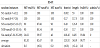
Comparative numerical results are reported in Table 2. The first row indicates the instance name and its characteristic parameters (T,N,P,K), respectively period of cyclic emission, router number, IP number, and message number. The other rows present the results for the three heuristics with their neighborhood size and two configurations of the ILP solver. For each method, are reported the computation time and the total length, averaged on a basis of 100 runs per instance. The test cases are ordered by increasing size. The N1 instance is the smallest one, whereas the N4 the larger one. The last two columns respectively report the average value over the whole benchmark set and the 95% confidence intervals computed based on standard deviation. We can observe that the three heuristics produce solutions with similar length values, then, of similar quality. A slight improvement of the computation time can be observed for ILS methods against IRS. However, there is place for improvement for the ILS methods, since as usual for heuristics [24], complete copy of data structures could be avoided by a better implantation of the local neighborhood operation. The ILP was solved using the GLPK¹ integer linear programming solver. Two configurations of the ILP solver are considered and the results reported in the last four rows in Table 2. In the two rows “first-sol”, are reported the values corresponding to the first admissible solution obtained during a run. This solution is not optimal. In the two rows “opt-sol”, are reported the optimal solutions found. Only the two smallest instances were solved successfully by the GLPK program within a reasonable amount of computation time, that was set to a maximum of 48h for the largest instances. It is worth noting that the ILP model generates a huge number of variables and constraints to be tackled by the solver as the problem size grows. As an example, the N3B instance case roughly produces 31 million variables with 5 hundred thousand constraints. According to the small instance cases N1 and N2 that were solved exactly, the heuristic method generates feasible solutions roughly at least 2000 times faster than the ILP solver. We think that these results highlight the contrast of behaviors when respectively dealing with an exact and heuristic method.

¹GNU Linear Programming Kit

Table 2: Comparative results on the whole benchmark set.

The two default parameter values of the neighborhood sample size and neighborhood size, respectively, were set empirically after a first round of experiments not reported in this paper. It appeared that increasing the sample size made the ILS-BI clearly worst performing, since it examines many more candidate neighborhood solutions at each pivoting operation. About the neighborhood size itself, i.e., the maximum number of paths suppressed/rebuilt at each move, we try now to better evaluate its impact. We diminish the neighborhood size, from actually all paths that can be suppressed (large neighborhood), to half of the paths suppressed (medium neighborhood), and to exactly 2 paths suppressed (small neighborhood). We perform a complete execution of the three heuristics on the whole benchmark set, executing 100 runs per instance, for each of the three neighborhood sizes. Average results are shown in Figure 8 within 95% confidence interval. The two graphics in the figure let us evaluate the trade-off between solution quality (length value) and computation time. The graph on the left shows that length values are rather similar. Since all confidence intervals overlap, the differences in the lengths look not statistically significant. On the contrary, some disparities appear between computation times, as shown in the right graph in the figure. The first point to note is the similitude of behaviors between the ILSBI and ILSFI methods as the neighborhood size diminishes. This is not surprising since the methods are similar and examine a relatively small sample in the neighborhood. The second point to note is the contrast of behaviors between ILS and IRS methods. While the former approach performs significantly faster with a large neighborhood size, the situation is inverted with a small neighborhood size since the latter becomes significantly faster than the former. This casts a light on the intensification/diversification tradeoffs into the methods. The ILS searches for improvements around a given pivot element which restricts the search region. But increasing the neighborhood size augments diversification. On the contrary, the IRS performs random steps in random directions starting from a given solution. This naturally increases diversification. But decreasing the neighborhood size restricts the search region. With regards to the trade-off between computation times and lengths, it seems that all configurations yield similar quality results, whereas fastest computation times occur for the IRS with small neighborhood, or ILS methods with medium or large neighborhood. Confidence intervals indicate that these last configurations are the best ones.

Figure 2: Impact of the neighborhood size on lengths and execution times.

The numerical results in Table 2 allow us to compare ILS-FI and ILS-BI regardless of the neighborhood size and considering simultaneously the time and the length, ILS-FI performances are the best on N1, N2 and N4. However, those of ILS-BI are the best on N3A. ILS-FI behaves better on small and large instances while ILSBI performs better on instances that we could describe as medium. This confirms the best behavior of ILS-FI on many instances. In these experiments, our main goal was to give an insight of the important contrast in computation time required when respectively dealing with exact and heuristic methods. We should mention that further work could adequately combine the benefit of both methods following the spirit of “matheuristic” approaches that aim at dealing with ILP acceleration according to the quick generation of feasible solutions by heuristic procedures. We expect that such adequate combinations could be studied in the future starting from the preliminary work presented in this paper.

4.3 Evaluation on random instances

We first detail the random instance generator, then we evaluate the local search approach on these randomly generated traffic configurations. The section also illustrates the designer’s problem of bandwidth decomposition and bridging the inaccessibility of many real-live problem instances.

4.3.1 The random instance generator

To evaluate the robustness of the method against a large range of traffic communication configurations, we have developed a generator of random instances. Based upon an application communication graph that specifies the inter-communications links opened between a set of IP components, the goal is to generate the quantity of packets that define the allocated bandwidth between each pair of sourcedestination nodes. In other words, given a set of K source-destination nodes (i, j) of a CKPP instance, the goal is to generate random packet quantities xi j in a way consistent with the cyclic nature of the problem. Since source-destination messages are emitted based on a temporal cycle of length T, two types of constraints are to be satisfied. They concern emitters and receivers to avoid trivially infeasible instances respectively. They state that the allotted T time-slots must be shared by emitters as well as by receivers. More formally, we state the problem of bandwidth decomposition as follows.

Let Π={1,2, . . .P} being the set of IPs, which may be either source or destination nodes. We define the application communication graph (ACG) as a matrix C = (c_i,j), 1 ≤ i, j ≤ P, such that c_i,j Є {0,1} whenever i ≠ j, and c_ii = 0 otherwise. An entry c_ij is such that c_{i j} = 1 if an open communication link exists from i to j, c_ij = 0 otherwise. Given an ACG, the model involves variables x_{i j} indicating the number of packets associated to each source-destination link (i, j). Let s be a lower bound on the number of packets emitted by a given source. The generation of traffic instances, that we call Traffic Injection Problem (TIP), consists in generating many and diverse random instances for the CKPP.

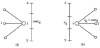
We are here concerned with the generation of many flow configurations of relatively good quality, rather than with necessarily generating a single maximum flow configuration. The quantity Σ_i,j c_ijx_ij is the total flow that is injected in the network during the period T. In order to measure the saturation level of the emitters as in [27], we define the message throughput (MT) as the quantity (Σ_i,j c_ijx_ij/ PT)×100, that is, the percentage of the emitted packets related to the available time-slots at each source node. Figure 3 illustrates the problem of instance generation on a simple case. In (a) the ACG is shown, whereas in (b) and (c) two optimal configurations of the traffic flow are shown. We should note that, with a threshold of s = 0, optimal solutions may be unsatisfactory since some IPs may have no packets to communicate, as in (b). The goal is rather to share and decompose the flow between emitters/receivers to allow to communicate, as in (c). It is worth noting that the maximum flow value first depends on the ACG structure, regardless of the NoC topology. As an example, the MT cannot exceed 66,6% in the ACG in Figure 3. This example illustrates how the guaranteed traffic approach constrains the bandwidths to be carefully settled.

Figure 3: An ACG (a), and two maximum traffic flow configurations (b-c).

To generate many random traffic instances, we proceed in two main steps as shown with Figure 4. First, as illustrated in (a), we randomly partition the receiver bandwidth between its related emitters. The random choices are done according to uniform sampling. The values obtained at each receiver node define the maximum amount of traffic that a related emitter node can send to that receiver. Second, as in (b), we adjust proportionally these maximum bandwidths at the level of each emitter, while trying to maximize the number of packets sent. At each step, a difficulty arises because traffic values are integer values rather than fractional values. Hence, fractional values are floored to their nearest integer, and the lost packets are randomly re-injected one by one to the different bandwidths, taking care of the maximum available time-slots for each emitter/receiver. The random choices also take care of the threshold s, in such a way that at least s packets are sent by each emitter node. For the experiments, this threshold is set to s = 2 packets, since messages contain at least a header packet followed by a data packet. Following part of the results in 3, we note that the MT is slightly inversely proportional to the size of T.

Figure 4: Random partition of a receiver bandwidth (a), adjustment of an emitter bandwidth (b).

4.3.2 Performances of local search against random instances

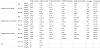
We evaluate the performance according to a wide range of random traffic configurations. Starting from the five real-life test cases and their respective communication graphs, we randomly generate new traffic values following the random process specified above. For each test case, we generate 100 new traffic instances with a threshold of two packets per message. Then we run the algorithm on these instances and evaluate the average value over these 100 runs. Results are presented in Table 3. Only the local search first-improvement is used. Two columns “MTreal” and “MT-rand” respectively report the message throughput of the real-life instances and of their random instances counterpart in average. The column “MT max” gives the maximum MT over the 100 generated instances. In addition to the execution time in seconds and length value, are reported the percentage of built paths and the percentage of admissible solutions found over the 100 runs. On the one hand, we can note that except the N4 test case, all the instances are solved successfully, and in a similar or shorter computation time than for the original reallife instances reported in Table 2. We can also note that, except for the N4 test case, the random MTs are all similar or inferior than those of the real-life instances. On the other hand, we can note that the N4 instance is never solved successfully, since only 94% of the paths are built on average, and no admissible solution was found. This should be explained by the higher random MT (39.97%) which is 50% higher than for the real case instance (26%).

Table 3: Results on random instances.

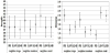
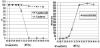
To evaluate to which extent the algorithm performs efficiently as a function of MT, we conduct new experiments. We progressively suppress packets from messages in order to gradually decrease the MT value. The results are shown on the two graphics of Figure 5. On the left part, are respectively shown the percentage of admissible paths and solutions found. On the right part, are indicated the related computation times. We can observe that 100% of the paths built are obtained below an intermediate MT level of roughly 30%. This means that the application can increase the volume of data exchanges from 26% initially to 30%, while preserving the actual NoC topology. As in a bin packing problem, packets are packed in the transmission links until some overload occurs. Hence, this study casts a light on the problem of network dimensioning, as the designer adjusts the packet quantities, while trying at the same time to guarantee contention-free routing, especially for large scale NoC.

Figure 5: Performances according to different levels of the traffic injection rate in the N4 NoC.