


1. Introduction
Population means and variances are generally estimated using sample estimates. If the parent population meets the requirements for normality, the distributional derivation of sample statistics such as the mean and variance are straightforward. However, the data generated from many real populations is typically bounded or significantly skewed. Weights and heights, for example, are strictly non-negative values, but are generally unbounded in the positive direction. Thus, a normal distribution characterized by a symmetric shape and infinite bounds may not be appropriate. Estimation from such data is traditionally addressed using large sample theory in conjunction with the Central Limit Theorem. While this solution allows normal theory to be applied to non-Gaussian populations, the amount of data necessary to implement such an approximation is often unavailable in real samples. Furthermore, the normal distribution assumed with this technique cannot account for any natural bounding which may occur.
By using the methods of Bayesian analysis and maximum entropy, procedures can be developed to produce probability distributions for sample statistics such as the mean and variance. These methods are non-parametric and require no distributional assumptions or sample size specifications. In addition, any naturally occurring bounds are inherently incorporated into the estimation process. Estimation can be carried out either independently for the mean or simultaneously for the mean and variance through the construction of a joint distribution. In this paper, the aforementioned procedures will be developed and demonstrated for the population mean and standard deviation.
2. Methods
In each of the following analyses, maximum entropy techniques will be used to determine the likelihood component required for a Bayesian posterior distribution given by:
where y is the parameter of interest, x is the observed data, and C is any prior information, p(x|y,C) and p(y|C) are the likelihood and prior probabilities constrained by C, respectively, and the denominator is a normalizing factor representing the total probability over the domain of the data, [a, b].
In 1948, Claude Shannon, working for Bell Telephone Laboratories on communication theory [1], found that the measure of uncertainty for a discrete distribution is:
for the probabilities pi. H(pi), or the entropy, was extended to the continuous case by Kullback and Leibler [2] as:
where a and b are the lower and upper bound on x, respectively, and m(x)=1/(b-a) is a reference distribution (Price and Manson [3]). While equation (3) provides a measure of the uncertainty for a specified distribution, it can also be maximized subject to known constraints on pi to identify the most uncertain distribution. Note that this process produces an entire distribution, not just a single probability point.
3. Distribution of the Mean
Nonparametric distributions for the mean and standard deviation were previously considered by Gull and Fielden [4]. While Bayesian analysis and maximum entropy were used in that work, the authors assumed convenient parametric forms (Gaussian) for the prior distributions, as well as, the reference distribution of the entropy. In this paper, the distributions are derived based solely on the assumptions that the relevant population moments exist and that the data are bounded.
For statistically independent data, the solution for a single data point can be found and generalized to a larger sample size. Let μ be the mean and x1 be a sample data point. From equation (1):
To determine the likelihood p(x1|μ), the entropy in the form given by equation (3) is maximized with the constraint:
resulting in the solution:
Normalizing equation (6) gives:
An analytical derivation of the LaGrange multipliers is not possible in this case. Since the solution must be found numerically and is computationally intense, it is convenient to solve the problem once for the generic bounds [-1, 1]. Any real problem can then be transformed to these bounds for an appropriate solution. The numeric solution for lambda can be obtained by substituting equation (7) into the constraint (5). Using this solution, the likelihood for each data point can be determined and then combined with a specified prior to derive the posterior distribution, p(μ | xn).
4. Joint Distribution of the Mean and Standard Deviation
The techniques given above can also be carried out for the two dimensional joint distribution of the mean and standard deviation. This requires two LaGrange multipliers which must be obtained numerically. As was the case with the mean, it is convenient to solve the problem once for the normalized bounds [-1, 1] and subsequently develop the distributions for real data sets after they are translated into this scale.
From Bayes theorem, the probability of μ and σ given the data x1 is:
and the entropy is:
Equation (9) is then maximized subject to the constraints:
The maximization problem solution is:
Using the normalization condition on p(x1 | μ, σ), λ0 evaluates to
Equation (14) has some interesting properties. First, the partial derivatives of λ0 with respect to λ1 and λ2, generate the constraint equations. Secondly, the equation is a “cup” function with a minima at the solution for the λi’s which can be found through numerical techniques.
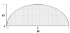
For convenience, the data bounds are again set to [-1,1]. Investigation of the probability plane of μ and σ will show that the domain for the probability function will be defined by a semicircular region of radius 1 which extends from -1 to 1 on the μ axis, and from 0 to 1 on the σ axis (Figure 1). This follows from the relationship between the mean and standard deviation. The probability function must be equal to 0 on and outside of these bounds.
All computations were written and carried out using standard ANSI C programs compiled under Linux 2.4. Program codes as well as a more detailed derivation of the distributions above may be found at . http://www.uidaho.edu/ag/statprog.
5. Demonstration
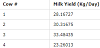
The techniques described above are demonstrated here using data collected from a nutritional dairy trial. The study was conducted as a cross-over design with two dietary treatments, two treatment periods, and four animals. For the purposes of this demonstration, only the control treatment (standard diet) will be considered. Given a sufficient wash out period between treatments, the data from each period can be combined resulting in n=4 data points (Table 1). Without making undo distributional assumptions, devices such as large sample theory and the Central Limit Theorem are clearly not useful in this case. Furthermore, the data to be analyzed, milk yield (kg/day), is bounded with a strict lower limit of zero and a conceptual upper limit of, say, no more than 50 kg/day.
6. Mean
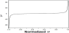
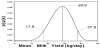
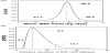
As was stated earlier, the LaGrange multiplier, λ, must be determined before the posterior distribution of the mean can be developed. To simplify this process, the problem was solved once for the general bounds [-1, 1]. This allows any real problem to be scaled to these generic bounds for determining λ and the associated likelihood. The problem is then rescaled back into the original units prior to obtaining the final probability distribution. The numeric solution for λ, as a function of the scaled μ, is shown in Figure 2. After computing the likelihood, a uniform prior for μ (the most uncertain distribution that can be used here) was assumed and applied to equation (1). The resulting posterior distribution for mean milk production is shown in Figure 3. The most probable value for μ was 28.8 kg/day with 95% credible bounds of [17.8, 37.6]. The distribution was slightly skewed towards zero due to the correct use of the bounding conditions that truncated milk yield at zero.
7. Joint Distribution for the Mean and Variance
Prior to estimation, values for the two LaGrange multipliers were determined numerically. Since the 2-dimensional problem was time consuming, a 100 x 100 matrix of λi values within the standardized semicircular domain for μ and σ was computed once and then stored. Estimation of the joint μ, σ distribution for this or any other data set could then be computed quickly without recalculating the λi values.
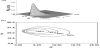
Assuming a joint uniform prior distribution for μ and σ over the domain of the data, a posterior probability surface was developed as shown in Figure 4a with a corresponding contour plot given in Figure 4b. The peak of the surface (μ = 28.8 and σ = 5.3 kg/day, respectively) represents the most probable values for both parameters while the surrounding contours form most credible regions. While these could be used for parameter inference, a simpler interpretation can be gained through integration of the surface. The resulting marginal distributions for μ and σ are given in Figure 5. Based on these marginal distributions, the 95% credible interval for μ and σ were [21.7, 35.4] and [3.3, 13.1], respectively. Although the most probable value for μ is the same as that given earlier, the interval is somewhat narrower. This is because more information was assumed for the joint estimation of μ and σ , i.e. that both the first and second moments of the data existed and also that they were bounded. Thus, the domain of possible distributions over which the entropy was maximized is reduced and the resulting marginal distribution for μ displayed less uncertainty.
8. Conclusion
Procedures have been developed and demonstrated which generate nonparametric probability distributions for the mean and joint meanvariance combination. Only minimal assumptions on the existence of relevant moments and bounds for the data are required for the purpose of estimation. The procedures are valid for non-Gaussian parent populations and do not rely on any sample size requirements.
Competing Interests
The authors declare that they have no competing interests.
Author Contributions
Both the authors substantially contributed to the study conception and design as well as the acquisition and interpretation of the data and drafting the manuscript.