2.1 Data collection in real environment

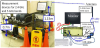
Measurements were carried out at a major railway station in Japan within both the 2.4 and 5 GHz bands. Measurements were conducted at the end of January 2017. The photograph of the measurement system on location and the configuration of the measuring device are depicted in Figure 1. The measurements were operated during a rush-hour in weekday evening (busy period) and around 05:00 in the morning (non-busy period) at a major railway station for about 30 minutes.

Figure 1: Measurement system and location.

The spectrograms of the measured data in busy period over the 2.4 GHz and 5 GHz bands are shown in Figure 2(a) and Figure 2(b), respectively. As shown in both figures, there are more wireless traffic over the 2.4 GHz bands than over the 5 GHz bands. On the other hand, even for the channels over the busy 2.4 GHz band, some channels have more traffic than others. The results reflect that the existing channel allocation methods are not fully efficient and a new method needs to be found to mitigate the usage imbalance. The spectrograms of the measured data in non-busy period also appear the similar property.

Figure 2: Spectrogram of the measured data at a railway station over 2.4 GHz and 5 GHz bands.

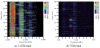
During the measurements, we also utilized a commercial sniffing software to capture all transmitted frames on Channel 1 (2.402-2.422 GHz) in the 2.4 GHz band and Channel 36 (5.17-5.19 GHz) in the 5 GHz band. From Figure 2(a) and Figure 2(b), we can find Channel and Channel 36 are one of the busiest channels in the 2.4 GHz and 5 GHz bands, respectively. Their header data was recorded using the software. Firstly, the frame arrival time, data-rate, and length were extracted. Then the number of data bits per symbol, bandwidth and standard (IEEE~802.11b/g/n) were obtained from the data-rate information based on the IEEE~802.11-2016 standards [15] using orthogonal frequency division multiplexing (OFDM). The frame duration was estimated from the required number of OFDM symbols after adding the MAC header with PHY preamble. The busy/ idle (B/I) sequence was then generated using a granularity of 9 μs per point following the current WLAN standards.

2.2 Statistics results of TOC

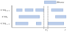
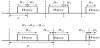
For data captured in a real wireless environment, it usually includes various application data with different traffic patterns. Therefore, it is generally difficult to realize an accuracy prediction of busy/idle duration, especially when busy/idle duration is long. In this paper, we limited our consideration for the application of simultaneous transmission over multiple wireless channels or bands where one long packet can be separated into several short packets and transmitted simultaneously to one receiver [11,12]. This technique requires the correct prediction of idle duration of each channel or band. In addition, due to simultaneous transmission, all channels or bands must have the time of coincidence (TOC) among them. The concept of TOC is shown in Figure 3 where three channels are used for the simultaneous transmission. The TOC is the idle duration of all channels with the same start point and end point as shown in Figure 3 with T_i. It is easy to understand that the more channels used for simultaneous transmission, the shorter the average duration of T_i is. This makes the prediction duration of channel status be shorter which reduces the difficulty of prediction design.

Figure 3: The time of coincidence (TOC) of multiple channels.

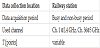
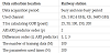
The distribution of T_i shows the prediction length of idle duration when considering the technique of simultaneous transmission using multiple channels. We show the statistic TOC results when two or three selected channels are used for simultaneous transmission over multiple channels in Figure 4(a) and 4(b). The specific channels and location information are listed in Table 1.

Figure 4: The time of coincidence (TOC) of multiple channels.

Table 1: Information of used data.

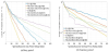
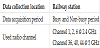
From both figures, we can find that the TOC of multiple channels decreases as the number of channels used increases. In addition, the TOC of data during non-busy period tends to be shorter than that of during busy period. For 2.4 GHz band, TOC duration of two channels are smaller than 100 points with about 60% and 40% for busy period and non-busy period, respectively. For TOC of three channels, the idle durations will be smaller than 100 points with about 25% and 45% for busy period and non-busy period, respectively. In addition, for TOC distribution over 5 GHz band, the TOC of idle durations is decreased with the increase of channel number. However, the TOC distribution between two channels and three channels is not largely different. The reason is that the wireless traffic over 5 GHz band is moderate or small regardless of busy and non-busy period.

From both figures, we can find that, the idle duration of TOC is limited within one or two hundred of points for both channels over 2.4 GHz band and 5 GHz band regardless of busy and non-busy period. The results also show that, for the usage of simultaneous transmission over multiple channels, the status prediction needs to be have a high accuracy performance for predicting the duration of one or two hundred of points ahead.

3.1 AR/ARI model

In statistics and signal processing, AR model is a representation of random process. Therefore, it is broadly used to describe certain time-varying processes in natural, economics, etc. The AR model specifies that the output variable depends linearly on its own previous and on a stochastic term (an imperfectly predictable term); thus the model is in the form of stochastic equation [16].

The notation AR(p) indicates an auto-regressive model with order p. The AR(p) model is defined as

$X_t=c+{\displaystyle {\sum }_{i=1}^p{\phi }_i{X}_{t-i}}+{\epsilon }_t,{\epsilon }_t\sim N(0,{\sigma }_a^2)$ (1)

where φ₁…φ_p are the parameters of the model, c is a constant and ε_t is white noise. In some cases, for the simplification, the constant term c is not included for usage. Therefore, the Equation (1) becomes as

$X_t={\displaystyle {\sum }_{i=1}^p{\phi }_i{X}_{t-i}}+{\epsilon }_t,{\epsilon }_t\sim N(0,{\sigma }_a^2)$ (2)

When using AR model for the prediction of status duration, the coefficient is calculated using training data so that they give the solution as the least squares for linear regression with Yule-Walker equation [16]. The predicted status duration $\widehat{X}(n)$ can be calculated as follows

$\widehat{X}(n)=-{\displaystyle {\sum }_{i=1}^p{\phi }_{i}X(n-i)},$

where $\widehat{X}(n)$ is the one-step predicted time-series data.

When time-series data is not a steady process, the efficient way is to take a difference operation on it and make it be a more steady one which increases the prediction performance. Let us using following equation to represent the i-th order difference operator on time-series data as

$X_{t-i}=L^i{X}_t$ (3)

Here the operator L is a lag for time-series data which transforms the data into one past element. For example, for one order difference operator on the input data X, its output ΔX_t can be represented as

${\Delta }^1{X}_t\equiv (1-L)X_t=X_t-X_t{}_{-1}$ (4)

In general, the stochastic process that can be made a steady process by taking the difference operation with d times is called the d-th order integrated process. Therefore, AR model using time-series data with d order integrated process is named as ARI (auto-regressive integrated) process with d-order difference and represented as ARI (p, d). Therefore, ARI model is just one of AR models. The whole process is identical to that of AR model but the time-series data is the one with d times difference operations for the coefficients calculation.

3.2 The relationship between busy/idle duration and COR

Till now, although there are many researches on the prediction of COR, it is difficult to use for the prediction of busy/idle duration because the resolution time T is long to second order which includes many busy/idle durations. However, when resolution T is small to μs order, the relationship between the COR and busy/idle duration can be easily decided. Therefore, we can employ the conventional COR prediction method for the prediction of busy/idle duration based on the relationships.

COR is the ratio of total channel occupancy duration to the resolution T which is calculated as

$\text{COR}=B_T/T$ (5)

where B_T is total channel occupancy duration during the T. According to Equation (5), the COR value is ranged as in [0,1].

COR value varies with the value of T. Therefore, the distribution of COR will be changed with different type if T is changed. Figure 5 shows the COR value is changed if the resolution duration T is different. Figure 6 shows the relationship between the COR and busy/ idle duration. We use Figure 5 and Figure 6 to explain our major idea of the proposal.

Figure 5: COR value with resolution duration T.

Figure 6: The relationship between the COR and busy/idle duration.

As shown in Figure 5, the COR value and its distribution are strongly related to the resolution duration T. The existed COR prediction research usually utilizes a large value T to get a stationary COR values for good prediction performance. However, a large T will include multiple busy and idle durations which is difficult to decide the start and end points of busy/idle duration.

The relationship between the COR and the busy/idle duration is shown in Figure 6. We can divide the relationship into two types. For type 1, if COR value is 1 or 0, it will be all busy or idle duration which can be directly decided. For some COR values among the (0, 1) as shown in Type 1 of Figure 6, using the previous COR value, either of two cases can be decided. If previous COR is not 0, the current waveform with COR as B_T/T is the left one of the Figure 6 with high probability. Accordingly, if the previous COR is 0, the current waveform with COR as B_T/T is the right one of Figure 6. However, for Type 2 where B_T is smaller than T or multiple busy durations are included in a resolution T, it is difficult to get the correct start or end points of busy/idle durations.

From Figure 6, we can also find that, if the resolution duration T is reduced to a small value, the ratio of Type 1 will be largely increased. Although large value T can get a stationary values for good prediction performance, here we use a small T to find an efficient way to recover the busy/idle duration from COR using existed low-complexity predictors.

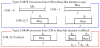
To show this, we utilize the captured data to calculate the ratio of Type 1 with the different value of T as shown in Table 2. The results are listed in Table 3(a) and 3(b). As shown in Tables 3(a) and 3(b), the ratio of Type I will be increased to more than 98% if T is smaller than 25 [points] for both data captured at busy period and non-busy period. Therefore, we can obtain good prediction performance on start and end points of busy/idle duration if COR prediction can be correctly realized using small T.

Table 2: Conditions for COR distribution.

Table 3(a): The ratio of Type 1 (Ch. 1 @2.4 GHz).

Table 3(b): The ratio of Type 1(Ch. 36 @5 GHz).

7.1 The performance of COR prediction

Figure 7 shows the COR prediction results using AR and ARI predictors with different value of T for data captured in busy period and non-busy period over 2.4 GHz and 5 GHz bands, respectively. Both figures show the CDF of absolute value of prediction error. For ARI predictor, we set the difference order as 1 for performance evaluation.

Figure 7: COR prediction performance of AR and ARI predictors (ARI: d = 1).

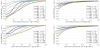
As shown in Figure 7, the prediction accuracy will be improved for both AR and ARI predictors with smaller value T than that of large T. The reason is that there are many continuous 1s or 0s with small value T which makes both predictors obtain good prediction accuracy. In addition, compared with AR predictor, ARI predictor can get better prediction performance than that of AR predictor especially for the data obtained from Ch. 1 at 2.4 GHz band at busy period as shown in Figure 7(a). The reason is that the busy and idle durations variate dramatically because of the wireless access from large user terminals at 2.4 GHz band during busy period. It can also be confirmed from the CDF of idle durations at Figure 4(a) and (b). When the scenarios are changed from large user access to small users access as from Figure 7(c) over 2.4 GHz band during non-busy period to Figure 7(b) and (d) over 5 GHz band during busy and non-busy period, the COR prediction difference between the AR predictor and ARI predictor is becoming small value. These results show that ARI predictor can have better COR prediction accuracy due to the difference operation of ARI when the captured data is not a steady process due to that more application patterns from more users access are included in the collected data.

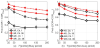
To further compare the COR prediction accuracy of both predictors, we use Figure 8 to show the probability of correct prediction for both predictors using data during busy and non-busy periods with the different T. As shown in both figures, the COR prediction accuracy is reduced when T is increased with the same reason as previous figure. In addition, the prediction accuracy of ARI predictor can be improved with about additional 40% to 50% than that of AR predictor for the data obtained from Ch. 1 at 2.4 GHz band at busy period.

Figure 8: COR prediction performance of AR and ARI predictors (ARI: d = 1).

To show the prediction performance of ARI predictor with different order d, we use Figure 9 to compare their results with d as 1, 2 and 3, respectively. As shown in the figure, ARI predictor with d = 1 can almost get better prediction accuracy than other difference order. The reason is that high difference order will make the data varied rapidly which decreases the ARI prediction performance.

Figure 9: COR prediction accuracy with different value d.

4.2 The performance of idle duration prediction

Finally, we show the prediction of idle duration using the COR prediction and the relation between the COR value and busy/idle duration as explained in previous section.

Here we use a new parameter named prediction success rate (PSR) to show the prediction performance between the calculated idle durations from predicted COR value and true idle durations. If the calculated idle duration is perfectly same or smaller than that of the original idle duration, we assume that prediction is successful.

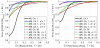
Figure 10 shows the PSR value using AR and ARI predictors with different value T. As shown in Figure 10(a), for the data captured at Ch. 1 over 2.4 GHz band during busy period, ARI predictor can provide better prediction accuracy with about over 20% higher than that of AR predictor when T is 25 points. Such difference of ARI and AR predictors is reduced to 8% when T is increased to 200 points. For the data captured for Ch. 1 over 2.4 GHz band during non-busy period, the accuracy improvement of ARI predictor can be 8% when T is short as 25 or 50 points.

Figure 10: The accuracy of idle duration prediction.

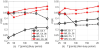
When channel has little users access such as data obtained in Ch. 36 over 5 GHz band in both busy and non-busy periods, the PSR of that using AR predictor has better results than that of ARI predictor. The reason is that, for this scenario, the merit of COR prediction using ARI is limited compared with that of AR predictor as shown in Figure 8. In addition, ARI predictor will cause more calculation error from the predicted COR when the channel status is changed to other one. Therefore, ARI based predictor can provide better prediction accuracy than that of AR based predictor when considering the data with large wireless access from users.

On the other hand, as shown in Figure 4(a) and (b), when simultaneous transmission over multiple channels is used, the TOC or common idle duration is short with high probability when the number of channel increases. This means that for most case, it is valuable even if the prediction algorithm can provide good prediction accuracy for short idle duration. Therefore, our proposed method can be used for the usage of simultaneous transmission over multiple channels or bands.