2.1 Mathematical Foundations

Terminology in this paper follows the one described by Kolda and Bader in [18]. Scalars are denoted by lower case letters, a. Vectors and matrices are described by boldface lowercase letters and boldface capital letters, respectively a and A. High order tensors are represented using upper case letter notation such as X.

The transpose matrix of A Є R^I×J is denoted by A^T.

The Moore-Penrose inverse of a matrix A Є R^I×J is denoted by A † .

X is called a n-way tensor if X is a n-th multidimensional array. It is expressed by

X is called a n-way tensor if X is a n-th multidimensional array. It is expressed by X∈ R I 1 × I 2 × I 3 ×...× I n

The square root of the sum of all tensor entries squared of the tensor X defines its norm.

‖ X ‖= ∑ j=1 I 1 ∑ j=2 I 2 ... ∑ j=n I n x j 1 , j 2 ,..., j n 2 (1)

The rank-R of a tensor X∈ R I 1 × I 2 ×...× I N is the number of linear components that could fit X exactly such that

X= ∑ r=1 R a r (1) ∘ a r (2) ∘...∘ a r (N) (2)

with the symbol ∘ representing the vector outer product.

The Kronecker product between two matrices A Є R^I×J and B Є R^K×L, denoted by A⊗B , results in a matrix C Є R^IK×KL.

C=A⊗B=[ a 11 B a 12 B ⋯ a 1J B a 21 B a 22 B ⋯ a 2J B ⋮ ⋮ ⋱ ⋮ a I1 B a I2 B ⋯ a IJ B ] (3)

The Khatri-Rao product between two matrices A Є R^I×K and B Є R^J×K, denoted by A⊙B , results in a matrix C of size R^IJ×K. It is the column-wise Kronecker product.

C=A⊙B=[ a 1 ⊗ b 1 a 2 ⊗ b 2 ⋯ a K ⊗ b K ] (4)

2.2 Non-Negative Paratuck2

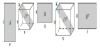
The Paratuck2 decomposition, [9], is well suited for the analysis of intrinsically asymmetric relationships between two different sets of objects. It represents a tensor X Є R^I×J×K as a product of matrices and tensors.

X= ∑ k=1 K A D k A H D k B B T (5)

A, H and B are matrices of size R^I×P, R^P×Q, and R^J×Q. The matrices D k A ∈ R P×P and D k A ∈ R Q×Q ∀k∈{1,...,K} are the slices of the tensors D^A Є R^P×P×K and D^B Є R^Q×Q×K. The latent factors p and q are related to the rank of each object set as illustrated in figure 1. The columns of the matrices A and B represent respectively the latent factors p and q, the matrix H describes the asymmetry between the p latent factors and the q latent factors. Finally, the tensors D^A and D^B represent the degree of participation, also called strength, for each of the latent factors, respectively p and q, according to the third dimension.

Figure 1: Paratuck2 decomposition of a three-way tensor with dimension notations.

To achieve the computation of the Paratuck2 decomposition, the following minimization equation has to be solved

min X ∧ ‖ X- X ∧ ‖ (6)

with X ^ the approximate tensor described by the decomposition and X the original tensor.

To solve equation 6, the Alternating Least Squares (ALS) method is used as presented by Bro in [10]. All of the matrices and the tensors are updated iteratively. To simplify the resolution explanation, we consider one level k of K, the third dimension of the tensor.

To update A, equation 5 is rearranged such that

X k =A F k  with  F k = D k A H D k B B T (7)

The simultaneous least square solution for all k leads to

A=X ( F † ) T  with { X=[ X 1 X 2 ... X k ] F=[ F 1 F 2 ... F k ] (8)

To update D^A, equation 5 is rearranged such that

X k =A D k A F k T  with  F k =B D k B H T (9)

The matrix D k A is a diagonal matrix which lead to the below resolution.

D (k,:) A = [( F k ⊙A) X k ] T  with  X k =vec( X k ) (10)

The notation (k, :) represents the k-th row of D (k,:) A .

To update H, equation 5 is rearranged such that

X k =(B D k B ⊗A D k A )h with { X k = vec( X k ) h= vec(H) (11)

which brings the solution

h= Z † x with Z=( B D 1 B ⊗A D 1 A B D 2 B ⊗A D 2 A ⋮ B D k B ⊗A D k A ) (12)

To update B and DB, the methodology presented for the update of A and DA is applied respectively.

In the experiments, we use the non-negative Paratuck2 decomposition leveraging the non-negative matrix factorization presented by Lee and Seung in [19]. The matrices A, B and H, and the tensors D^A and D^B are computed according to the following multiplicative update rule.

{ a ip ← a ip [X F T ] ip [A(F F T )] ip ,F= D A H D B B T d pp a ← d pp a [ Z T X] pp [ D A (Z Z T )] pp ,Z=(B D B H T )⊙A h pq ← h pq [ Z T X] pq [H(Z Z T )] pq ,Z=B D B ⊗A D A d qq b ← d qq b [XZ] qq [ D B ( Z T Z)] qq ,Z=B⊙ ( H T D A A T ) T b qj ← b qj [ X T F T ] qj [B(F F T )] qj ,F= (A D A H D B ) T (13)

with

{ X=[ X 1 X 2 ... X k ] X=vec(x) (14)

The non-negative multiplicative update rule helps to better calibration of LTSM since it uses the elements of the tensor decomposition as a starting point. Hereinafter is the complete algorithm of the non-negative ALS Paratuck2 resolution.

Algorithm 1 Non-Negative ALS Paratuck2 with P and Q latent components for a tensor X of size I × J × K

1. procedure NN-PARATUCK2(X, P , Q)
2. random initialization A Є R^I×P, H Є R^P×Q, B Є R^J×Q
3. set D k A ∈ R P×P and D k B ∈ R Q×Q equal to 1 for k = 1,...,K
4. X = [X₁ X₂...X_k]
5. x = vec(X)
6. repeat:
7. a ip ← a ip [X F T ] ip [A(F F T )] ip ,F= D A H D B B T
8. d pp a ← d pp a [ Z T X] pp [ D A (Z Z T )] pp ,Z=(B D B H T )⊙A
9. h pq ← h pq [ Z T X] pq [H(Z Z T )] pq ,Z=B D B ⊗A D A
10. d qq b ← d qq b [XZ] qq [ D B ( Z T Z)] qq ,Z=B⊙ ( H T D A A T ) T
11. b qj ← b qj [ X T F T ] qj [B(F F T )] qj ,F= (A D A H D B ) T
12. until maximum number of iterations or stopping criteria satisfied

2.3 Latent LSTM predictions

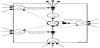
Based on the notation of Sak et al. in [20], LSTM contains memory blocks in the recurrent hidden layer. Each memory block is connected to an input gate and an output gate. Similarly to RNN, the input gate plays the role of the input activation of the memory cells. The output gate is in charge of the flow of cell activations into the rest of the network. In addition, a forget gate is added to the memory block since Gers, Cummins and Schmidhuber presented it in [21]. The forget gate allows the reset of the cell’s memory depending on the information received through the input gate. If we consider the input sequence denoted by x such as x = (x₁,...,x_T), the output sequence denoted by y such as y = (y₁,...,y_T) for a sequence of events from t = 1 to t = T. The mapping between x and y for all network unit activations within LSTM is described by the set of equations (15). The activation of the input gate is denoted by i_t, the candidate value for the states of the memory cells by C ˜ t the activation of the memory cells forget gates by f_t, the memory cells new state by C_t, the value of their output gates by o_t and the outputs of the output gates by h_t.

{ i t =σ( W i x t + U i h t−1 + b i ) C ˜ t =tanh( W c x t + U c h t−1 + b c ) f t =σ( W f x t + U f h t−1 + b f ) C t = i t ∗ C ˜ t + f t ∗ C t−1 o t =σ( W o x t + U o h t−1 + V o C t + b o ) h t = o t ∗tanh( C t ) (15)

In the set of equations 15 at time t, x_t stands for the memory cell layer, W_k and U_k with k= {i, c, f, o} for the weight matrices and b_k for the bias vectors. In the model used for the experiments, the activation of a cell’s output gate is independent of the memory cell’s state C_t such that V₀ = 0. The main advantage by fixing V₀ = 0 is the ability to perform faster computation, especially on large datasets.

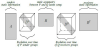
With regards to figure 1, the tensors D^A and D^B collects data about the tensor factorization related to the third dimension, which is very often the time. It means that the evolution of each groups, or clusters, characterized by the latent factors P and Q of the TD contained in the tensors D^A and D^B can be modeled using LSTM. More precisely, LSTM is calibrated on the historical data of the tensors D^A and D^B to predict afterwards the future evolution of each P and Q groups contained in the tensors D^A and D^B as illustrated in figure 3.

Figure 2: Overview of a LSTM memory cell. In our model, the activation functions g and h are described by tanh, and f is the forget gate.

Figure 3: Overview of LSTM training and predictions on the tensor D^m Є R^L×L×K with m= {A,B} and L= {P,Q}.

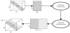
Only the diagonals of the tensors D^m with m = {A, B} contain numbers. Therefore, the tensors D^m Є R^L×L×K can be reduced to a matrix, E Є R^L×K. The notation L = {P,Q} denotes the latent factors of the Paratuck2 TD. Data contained in E is then used to train LSTM before performing the predictions on an interval Є related to the third dimension K. The resulting matrix of size R^L×(K+Є) gathers the historical data of each latent component L as well as the predicted values. A new tensor denoted by D ˜ m of size R^L×L×(K+Є) is built. The methodology is applied on both tensors D^A and D^B for the same Є. Consequently, the Paratuck2 TD is linked to historical data and predicted data.

3.1 Application to Smart Contracts

Smart contracts activities have been extracted from the Ethereum platform. The data was collected starting 1 January 2016 and ending 1 July 2016. Through the collection process, different data types have been stored, such as the hash key, the sender accounts, the receiver accounts or the blockheights. For the considered six months period, more than 5 millions of transactions have been made. This accounts for an average of 26 transactions per sender account and 18 transactions per receiver account.

In the data set, some smart contracts only relate to one transaction, payment or reception. Such behavior is difficult to predict, and should be considered as unexpected behavior. Our aim is to predict future interactions based on exchanges that already happened. Consequently, only the 1% most active smart contracts have been kept in the training set for their regular activities. This represents a list of 100 smart contracts sending an Ether amount, and a list of 200 smart contracts receiving an Ether amount from the sender contracts.

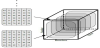
The features extracted from the dataset are well suited for a tensor representation. Two tensors denoted by X Є R^I×J×K are built from the Ethereum data. The first dimension, I, lists the sender accounts, the second dimension J, the receiver accounts and the third dimension, K, the time. For each tensor, the interaction between a sender and a receiver is represented by the amount of Ether exchanged at a time. The dense tensor is built based on figure 4. The size of the tensor is R100×200×50. The tensor is decomposed to highlights the latent component over time. Then, LSTM latent predictions are performed.

Figure 4: Three way tensor containing Ether amount exchanged between different smart contracts.

As illustrated in figure 5, the information evolving over time is contained in the tensors D^m with m= {A, B}. The matrix A gathers static information regarding P senders groups and the matrix B static information regarding Q receivers groups. The matrix H contains the asymmetric information between the P and the Q latent factors which have been set to respectively to 20 and 30. As a result, the LSTM network is trained on D^m for the sender and the receiver activities predictions.

Figure 5: Paratuck2 decomposition applied to smart contracts profiling. The model training and predictions are applied on the tensors D^A and D^B.

3.2 Predictions results

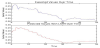
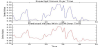
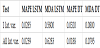
Figures 6 and 7 show the difference between the true experimental data and the predictions for one rank of the tensors D^A and D^A. The LSTM predictions of smart contracts activities are close to the one observed in the tensor decomposition of the complete true dataset. It means LSTM is appropriate for the modeling of the smart contracts having regular exchanges. To further quantify the accuracy of LSTM predictions, statistical tests are performed. The mean absolute percentage error (MAPE) and the mean directional accuracy (MDA) are computed betwen the predictions and the true data set. A third measure, the Jaccard distance, is also evaluated. As a benchmark for LSTM predictions, the results are compared to the predictions performed by a Decision Tree (DT).

Figure 6: Paratuck2-LSTM applied to smart contracts profiling. This simulation highlights training and predictions on one latent component of the tensor D^A.

Figure 7: Paratuck2-LSTM applied to smart contracts profiling. This simulation highlights training and predictions on one latent component of the tensor D^B.

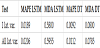
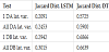
Tables 1 and 2 highlights similar MAPE results for both LSTM predictions and DT predictions. Differences are not significant. On the other hand, the MDA score is lot higher, around a factor 7, for LSTM predictions than for DT predictions. It means the LSTM predictions are able to better reproduce the variations observed in the smart contracts activities through time than the DT predictions. From these first statistical tests, we can observe that the LSTM model is able to reproduce the changes over time of smart contracts activities. It outperforms the decision tree benchmarking algorithm. In addition, the Jaccard distance is computed to underline the distribution divergence between the predictions and the true experimental data. In table 3, it can be observed that LSTM predictions are significantly closer to the true experimental distribution than DT predictions. All LSTM Jaccard distances are within the range 0.20 and 0.30 while the DT Jaccard distances are between 0.57 and 0.69. LSTM Jaccard distances are between 2 to 3 times lower than the DT Jaccard distances. It confirms the MDA scores in tables 1 and 2.

Table 1: Tests to assess the accuracy of LSTM predections on tensor D^A. Predactions are challenged by a decision tree (DT).

Table 2: Tests to assess the accuracy of LSTM predections on tensor D^B. Predactions are challenged by a decision tree (DT).

Table 3: Jaccard distances to assess the accuracy of LSTM predactions. Predactions are challenged by a decision tree (DT).

From the highlighted results, the combined approach of Paratuck2- LSTM delivered good results, validated visually and statistically. It outperformed the DT benchmarking for predictive analytics on several statistical criteria including the MDA and the Jaccard distance.